Scenario Planning and Analysis
 |
Analyst is designed to support iterative scenario development and analysis. The tutorials in this section take you through essential features for building and analyzing scenarios to represent and compare land use and policy alternatives.
Edit the Base Canvas
Generating the Base Canvas involves cleaning, compiling, and processing geographic and tabular data from a number of sources, including parcel data and multiple census datasets. Given the automated nature of this process, and the potential of inaccuracies in source data, you may find areas where the Base Canvas does not reflect existing development accurately.
To address any discrepancies, you can edit features of the Base Canvas to change their land use type and, optionally, their attribute values. In either case, changes are carried forward to the Base Canvas across all scenarios in your project. In this tutorial, we'll walk through editing the Base Canvas, and reverting features to their original base condition.
Data Layers | Features |
Learn to Edit the Base Canvas
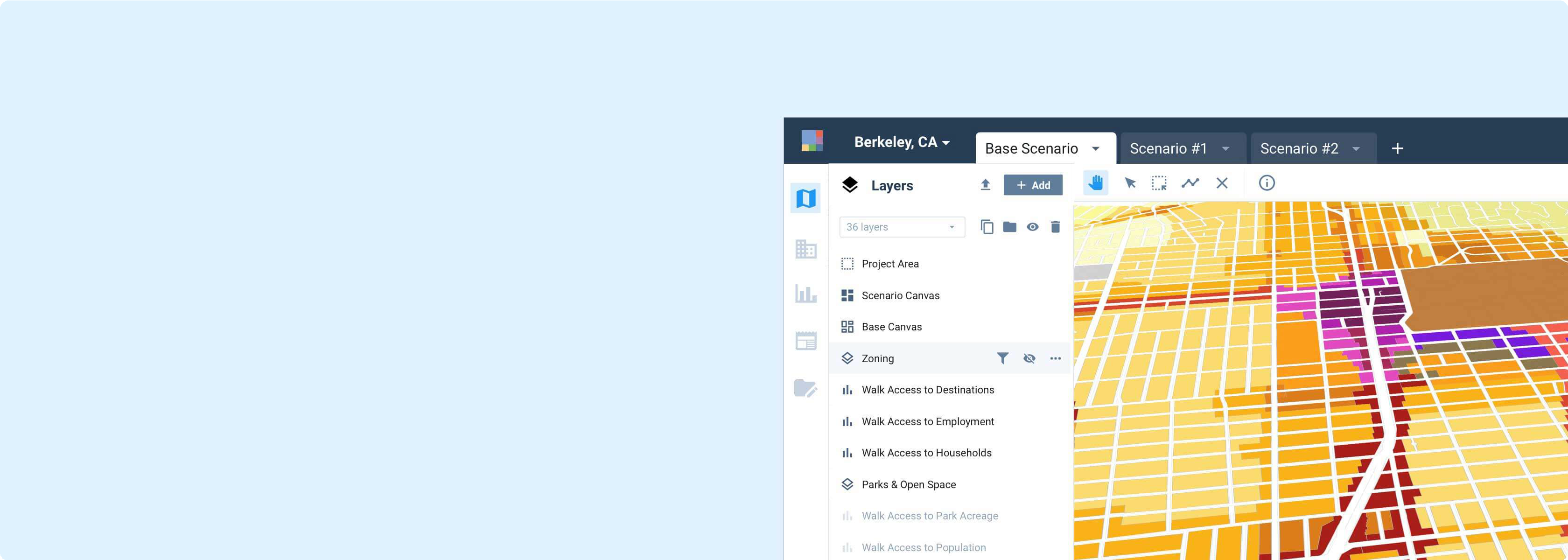
Select the Base Scenario tab.
Click the Build icon
 in the Mode bar. Alternatively, you can access the Base Canvas editing controls by activating the Base Canvas layer and selecting the Build tab in the Layer Details pane.
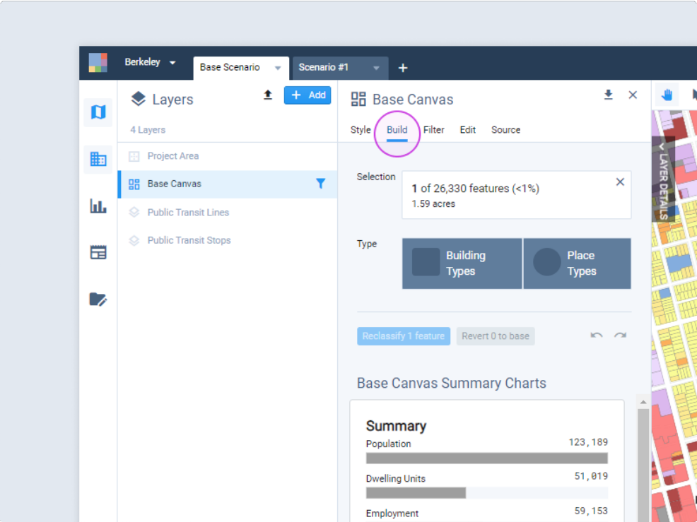
Accessing the Base Canvas editing controls
Select one or more features on the Base Canvas to reclassify. You can select features using the manual selection tools, or apply filters and/or joins to select features based on particular criteria. Details about your selection, including the number of features selected and their associated land area (in acres), will appear in the Selection control.
As an example for using filters, you could apply one to the Land Use Type (L4) column to identify parcels with "Blank Data"—indicating that the source data did not include sufficient information for a land use classification. It may be useful to review these features. Similarly, you could use an L4 filter to identify parcels classified as "Vacant." (In these cases, the Zoom to selection tool [icon] can help in finding the features on the map.)
For our example, we'll create a manual selection using the Point Selection [icon] tool. While redevelopment of these parcels has in fact been planned but not yet completed, for the purposes of our example we'll assume that it has been, and we want this to be reflected in the Base Canvas.
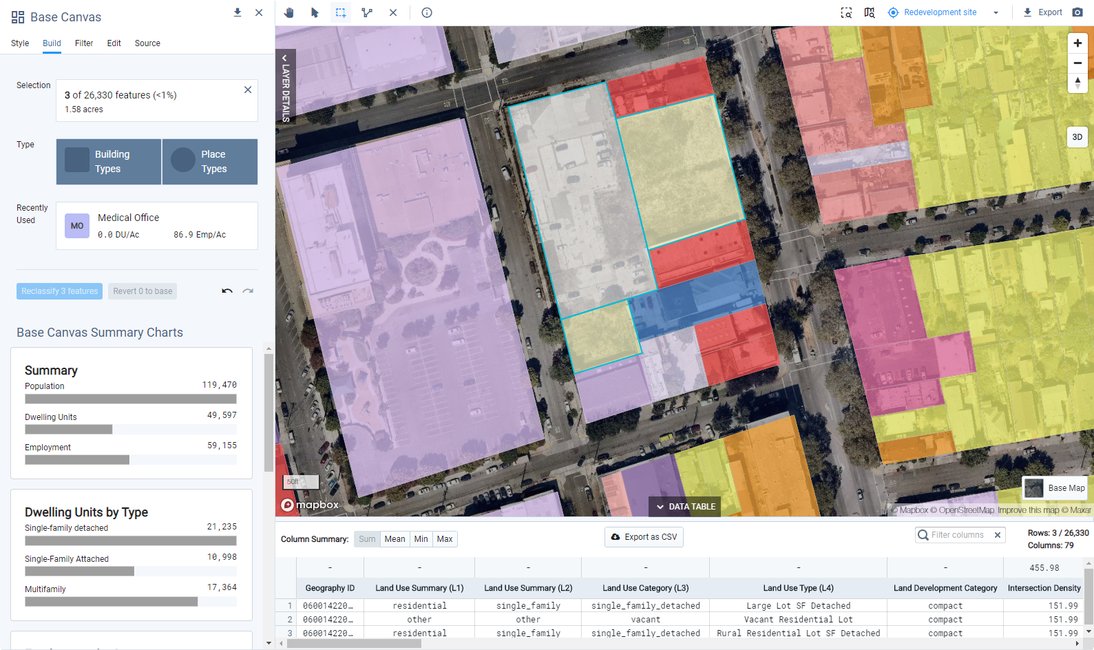
A selection of parcels to be reclassified
Click the Building Types button to open the type selection window. For our example, we're selecting a Building Type since our project uses a parcel canvas. The Building Type selection window will appear.
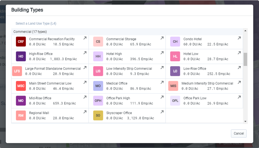
Building Types selection window
Select a type to reclassify with. The menu entry for each type indicates the residential and employment densities. You can click the expand arrow icon in the upper right corner to see more details. For our example, we'll select the Medical Office Building Type, a custom type created to align with plans for the site.
Review the values corresponding to your selection. The value options indicate the dwelling unit (DU), population, and employment counts associated with the selected features using either the new type, or as originally designated in the Base Canvas. You can use this information to decide whether to reclassify and update the values, or reclassify in type designation only.
We can see that, using the new Building Type, the selected features would accommodate 138 employees, and no dwelling units or population. The original base values include two dwelling units, five people, and zero employees.
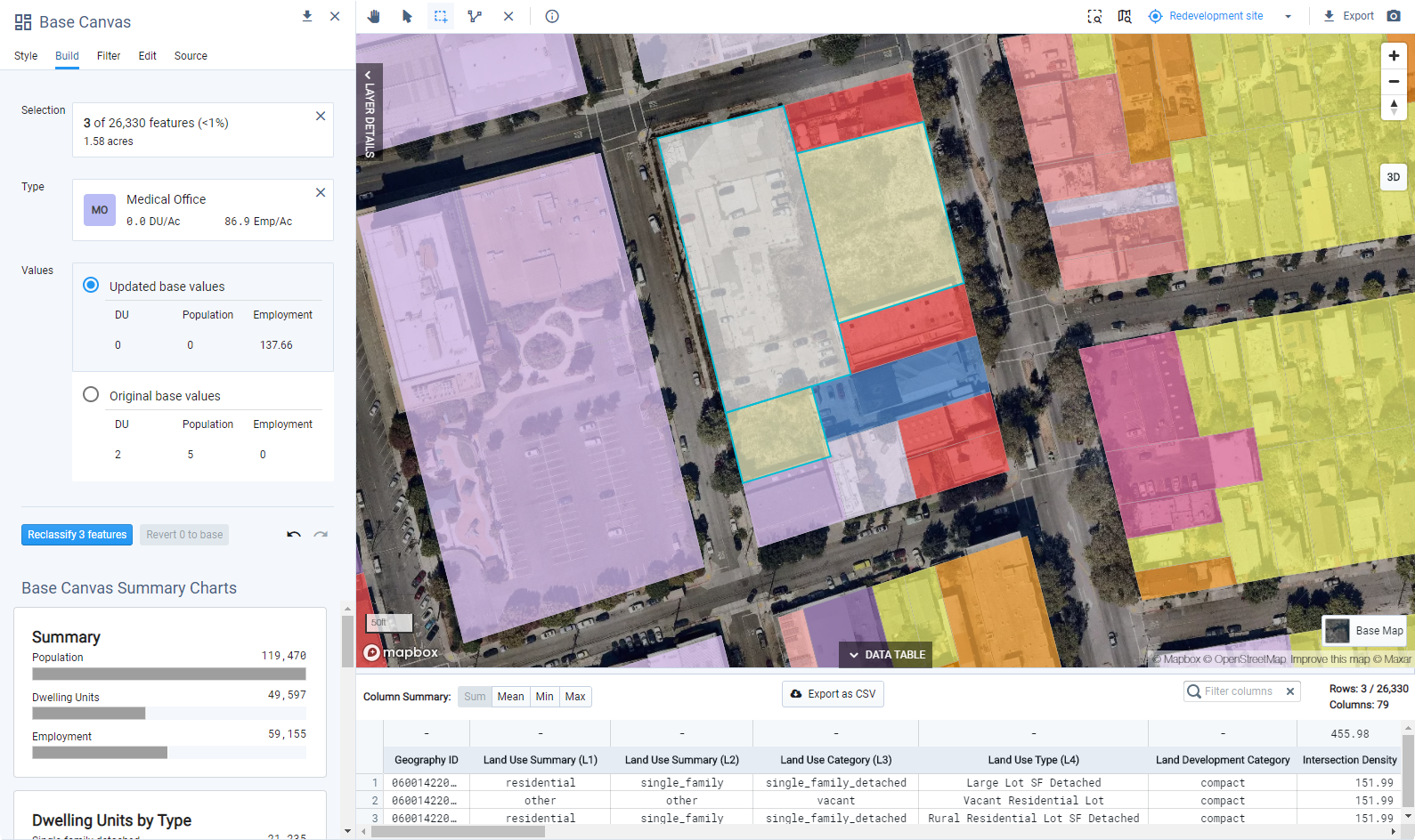
Select Updated base values to reclassify the land use of the Base Canvas and update values. For our example, we do want to update the base values. If you instead wanted to reclassify the land use of the Base Canvas without updating values, you could select Original base values. This would update the land use designations for the L1, L2, L3, and L4 columns according to the selected type, while maintaining the original values from the Base Canvas for DU, population, employment, and all other associated development characteristics.
Click the Reclassify 3 features button. A confirmation dialog appears. If you confirm, the features will be reclassified accordingly. The reclassification will be reflected in the scenario canvas summary charts, on the map, and in the scenario layer data table.
Editing the Base Canvas affects all scenarios because growth is allocated relative to the Base Canvas. Each time you reclassify features, Analyst updates all scenarios to reflect new values for the base, increment, and endstate as summarized in reporting charts and represented in the scenario layer. Depending on the number of features you are reclassifying, the scenario updates may take some time.
Editing the Base Canvas also renders any prior analysis runs as out of date. You will need to re-run analysis after reclassifying features and updating their values. The status as to whether results are current or outdated is indicated for each module in Analysis and Report modes.
Use the Undo
 or Redo
  controls to make sequential changes. The undo and redo arrows apply to your sequence of past actions, independent of the features that are currently selected. If at any point you need to return features to their original base condition, use the Revert to base control described in the next set of steps.
Revert Features
Reverting returns features to their original base condition, effectively clearing any past reclassifications for selections of features. Undo and redo, by contrast, are applied to your sequence of past actions independent of the features that are currently selected.
Select any features on the map that you want to revert to the original base values. The Revert x to base button will indicate the x number of features in your selection that have been reclassified in any prior actions.
For our example, we'll revert the features that we reclassified previously.
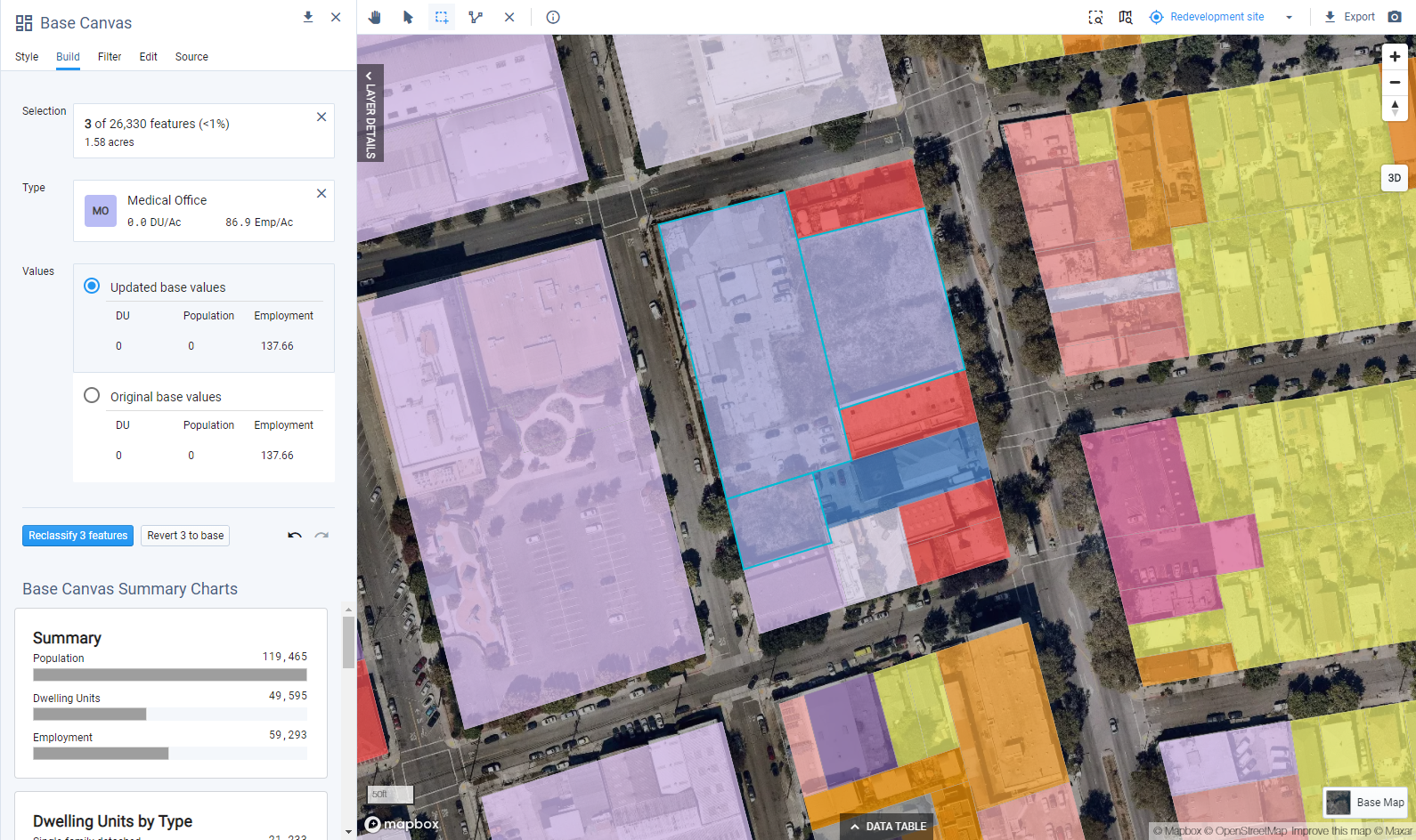
Click Revert 3 to base. This will reset the features to their original base condition, including land use classifications and base values. Any features that have not been reclassified previously will be unaffected by the revert action.
When complete, the effects of reverting features will be reflected in the Base Canvas Summary Charts, as well as any scenarios.
Again, editing features in the Base Canvas affects all scenarios because growth is allocated relative to the Base Canvas. Each time you reclassify or revert features, Analyst will update all scenarios to reflect new values for the base, increment, and endstate as summarized in reporting charts and represented in the scenario layer. Depending on the number of features you are reverting, the scenario updates may take some time.
Editing the Base Canvas also renders any prior analysis runs as out of date. You will need to re-run analysis after reverting features. The status as to whether results are current or outdated is indicated for each module in Analyze and Report modes.
Create a New Component
Building and Place Types are used to classify existing development and allocate growth via the scenario development process. Analyst's default types are based on studies of development across the United States, and cover a range of potential development patterns—from mixed-use centers, to residential areas, to focused employment and industrial areas—and the buildings within them.
Reviewing the set of types that you'll use in a project, and Library Settings for variables such as household sizes, is a fundamental first step in scenario development. For most planning projects, Building and/or Place Types should be created or adapted to best represent local conditions, plans, or zoning regulations. While there is a learning curve to understanding how to specify types—many inputs for specific attributes about households, employment, and building and site characteristics are required to support robust impacts analysis—the ability to tailor them for your projects can yield more grounded scenarios.
In this tutorial, we'll create a new Component using the Land Use Type Manager. As part of the process, we'll look into Library Settings, which include project-wide variables that affect population and employment density. We'll create a Building Type, then a Place Type, in subsequent tutorials.
For more information about land use types, the Land Use Type Manager, and Library Settings, see the Land Use section of the Features documentation.
Data Layers | Features |
None |
You can add a new component or type to your library in either of two ways: by creating it from scratch, or as a copy of an existing Component or type which you then edit. For our example, we're going to first create a new Component.
Enter Manage mode. Click the Manage icon
 from the left-hand menu bar.
From Manage mode, navigate to the Components screen. Components can represent individual buildings, or elements such as parks and parking lots. We're going to create a Component based on a real-world building.
Click the + Add new button. A new Component window appears. We'll step through the necessary inputs as we continue.
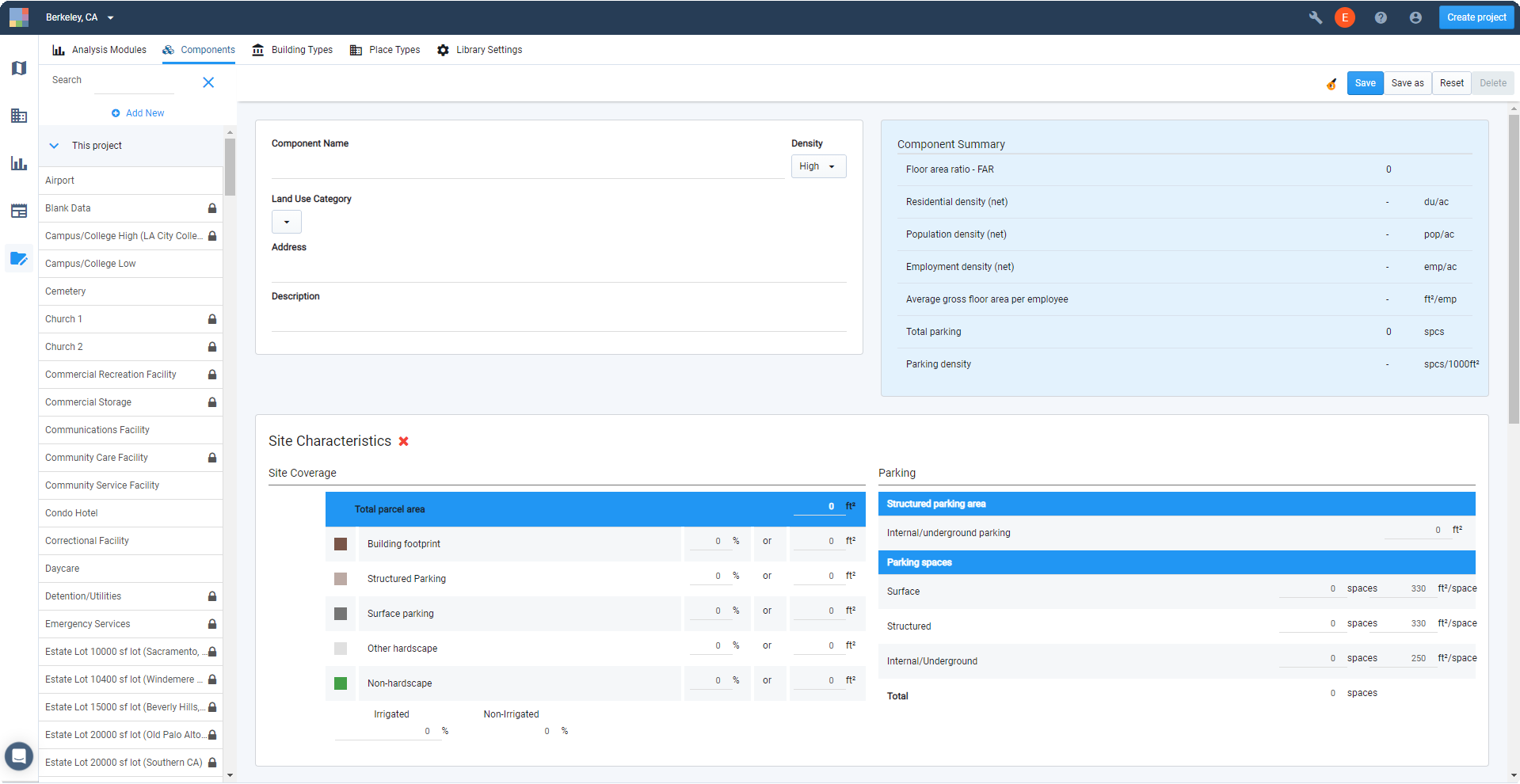
Enter Component information. The Component Information panel contains basic information for identifying and categorizing the Component.
Component Name – Names can be as descriptive as you like. If you're creating a number of local Components, it can be useful to add an identifier to their names so that you can easily filter your Components list using the search box.
Density – Refers to the building density category. Options include High, Medium, and Low. These categories are used to differentiate variables for the employment density of commercial floor area, as managed in Library Settings.
Land Use Category – Refers to the Level 3 (L3) land use category. Select the L3 category that the Component should be associated with. (See Land Use Hierarchy for information on the land use levels.)
Address – The address of the Component, if applicable. This field is optional.
Description – A description of the Component. This field is optional.
Building Types – This is a list of the Building Types in which the Component is included. The list is automatically generated. The Building Type names link to the Manage screen for the Building Types.
The inputs for our new Component example are shown below.
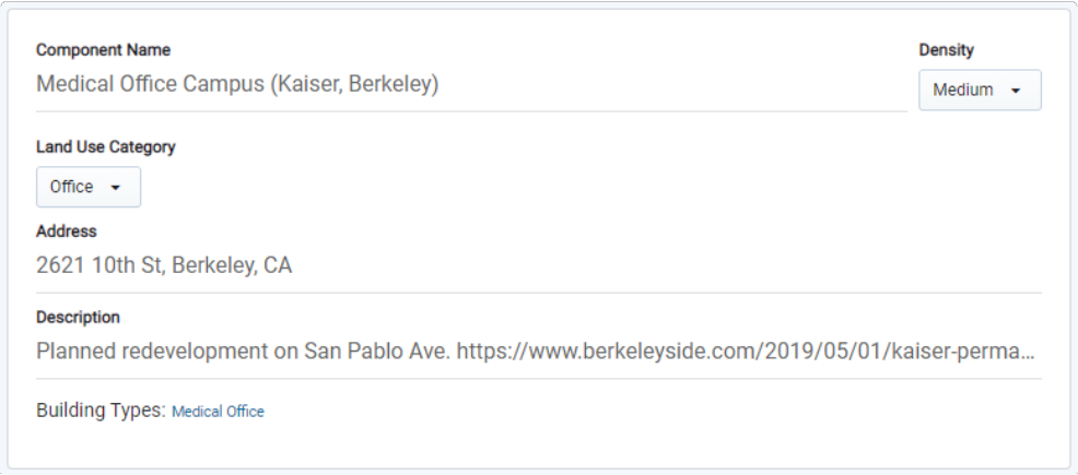
Component Information panel
Enter Site Coverage details. The Site Coverage section of the Site Characteristics panel describes how the land area of a Component is distributed. Each of the constituent site area values is expressed as either an absolute value or a percentage of total parcel area. The values are tethered such that the model automatically populates one or the other depending on a given input for either.
Total parcel area – The area of the parcel or site. Components represent development on parcel or "net" land area only—that is, area not inclusive of rights-of-way or other infrastructure components.
Building footprint – The land area covered by the ground floor of the building, expressed as an absolute value or as a percentage of total parcel area.
Structured parking – The land area covered by any dedicated parking structures on site, expressed as an absolute value or as a percentage of total parcel area. This should not include area attributed to internal or underground parking, which by definition fall within the building footprint.
Surface parking – The land area covered by surface parking, expressed as an absolute value or as a percentage of total parcel area. This value is tethered to the number of surface parking spaces and the assumed area per space as specified in the Parking section. If either the surface parking area or number of spaces is edited, the other number is adjusted accordingly.
Other hardscape – The land area covered by walkways, patios, and any other type of impermeable hardscape, expressed as an absolute value or as a percentage of total parcel area.
Non-hardscape – The land area not covered by hardscape, expressed as an absolute value or as a percentage of total parcel area. This can include landscaped areas, bare land, or any other permeable area.
Irrigated / Non-irrigated – The percentage of non-hardscape area that is assumed to be irrigated. The percentage of non-irrigated area is calculated automatically on the basis of the irrigated area input.
Overallocated / Unallocated – A value, as shown below, that appears if the total of the constituent site areas as specified falls above or below the total parcel area. Use this value to correct the site area allocations. The Component will not be valid for use if there is any overallocated or underallocated area.
For our example, we have entered the values below based on given development information.
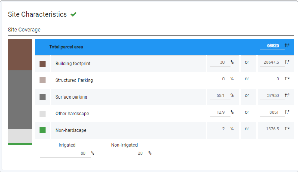
Site Characteristics panel > Site Coverage section
Enter Parking details. The Parking section of the Site Characteristics panel describes the amounts of parking by type included in the Component.
Internal/structured parking area – The total area dedicated to internal or underground parking, which is defined as parking that is located in garages within the structure of a building. This area is not accounted for as building area. The value is tethered to the number of internal/underground parking spaces and the assumed area per space.
Surface parking spaces – The number of surface parking spaces, and assumed area per space. These values are tethered to the surface parking area value in the Site Coverage section. If either the surface parking area or number of spaces is edited, the other number is adjusted accordingly. Note that, depending on the parking condition (e.g., parking lots vs. individual spaces on a property), the assumed area per surface parking space can be inclusive of drive aisle area.
Structured parking spaces – The number of parking spaces in a standalone structured parking garage, and assumed area per space. If any number of structured parking spaces are specified, a value for structured parking site area (equivalent to the footprint of a parking structure) should also be specified. The assumed area per structured parking space should include drive aisle area.
Note that structured parking can either be bundled with a building within a Component, or accounted for separately as a standalone Component.
Internal/Underground parking spaces – The number of internal or underground parking spaces, which are defined as parking located in garages within the structure of a building or underground, and assumed area per space. The value is tethered to the total area for internal/underground parking.
For our example, we have entered the values below based on given development information.
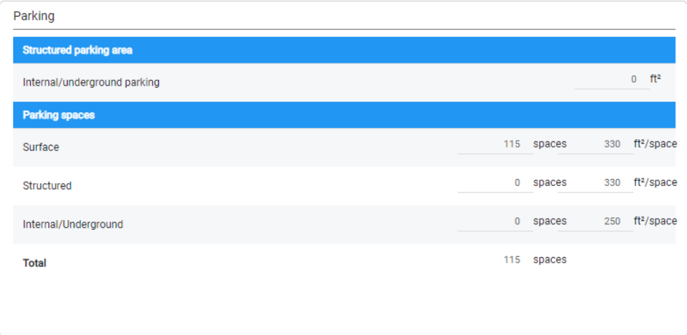
Site Characteristics panel > Parking section
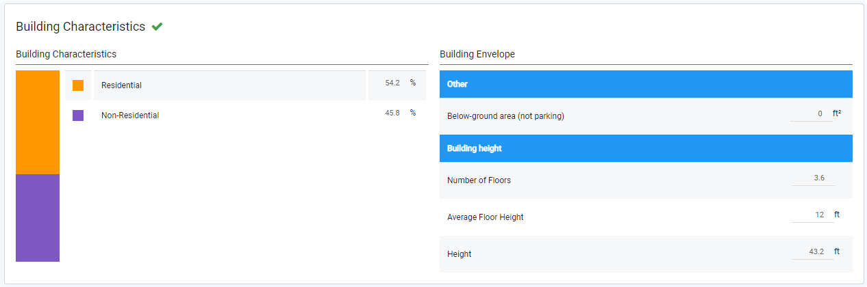
Enter Building Characteristics details. The Building Characteristics panel describes building floor area and how it is distributed, along with building envelope characteristics.
Total floor area (gross) – The total gross building floor area of the building(s) on site. Gross floor area is inclusive of internal hallways, lobbies and other common areas; space for building systems; and other non-leasable space. Net-to-gross floor area factors for residential and non-residential building area are set in the Floor Area Allocation panel.
Residential – The amount of gross floor area dedicated to residential uses, expressed as an absolute value or as a percentage of total floor area.
Non-Residential – The amount of gross floor area dedicated to non-residential uses, expressed as an absolute value or as a percentage of total floor area.
Our example building is purely non-residential, so we have entered the values below.
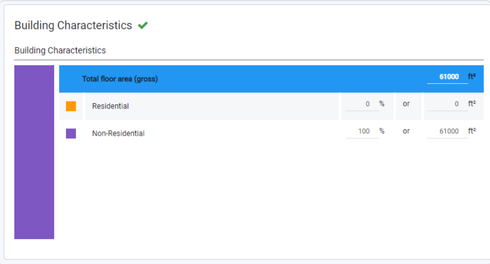
Building Characteristics panel - Parking section
Enter Building Envelope details. The Building Envelope section of the Building Characteristics panel contains attributes describing building height and below-ground area.
Below-ground area (not parking) – The amount of area dedicated to basements and other below-ground space, and not used for parking. This value is not associated with the values for gross floor area, so any value entered here is informational.
Number of Floors –The number of floors or stories in the building. This value is tethered with average floor height and building height such that building height is the product of the number of floors and average floor height. The number of floors is not associated with values for building square footage, site coverage, or Floor area ratio (FAR).
Average Floor Height – Average floor-to-floor height for the building. This value is tethered with the number of floors and building height such that average floor height is the quotient of the building height and number of floors. Floor height is not associated with values for building square footage, site coverage, or FAR.
Height – The height of the building. This value is tethered with the number of floors and average floor height such that building height is the product of the number of floors and average floor height. Building height is not associated with values for building square footage, site coverage, or FAR.
For our example, we have entered the values below based on height information we obtained.
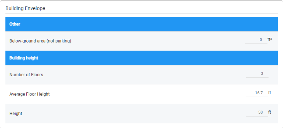
Site Characteristics panel > Building Envelope section
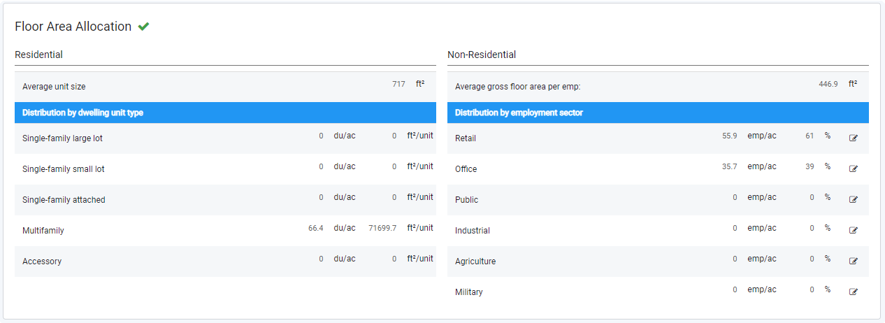
Enter Residential Floor Area Allocation details. The Residential section of the Floor Area Allocation panel describes how residential building area and dwelling units are distributed among dwelling unit types.
Gross floor area – The amount of gross floor area dedicated to residential uses. The value is set in the Building Characteristics panel and displayed here for reference.
Net floor area – Includes two values: a net floor area percentage and the resulting total net residential floor area in the building. Net, or leasable, floor area is calculated as the product of the net floor area percentage (also known as a net-to-gross ratio) and gross floor area. For single family building types, the net floor area percentage is typically 100%, while that for multifamily building types with internal hallways and common areas is lower.
Distribution by dwelling unit type – Inputs for each dwelling unit type include net floor area, number of units, and average unit size. The values are tethered such that net floor area is the product of the number of units and average unit size. Average unit size is expressed in terms of net floor area. The net floor area across all types must add up to the net floor area value for residential building area as specified above.
Single-family large lot – Analyst defines large lot homes as those with lot sizes of 5,500 square feet and above. The distinction between large and small lot single family homes supports the use of differentiated assumptions for household size, as well as analysis assumptions for energy and water use.
Single-family small lot – Analyst defines small lot homes as those with lot sizes under 5,500 square feet. The distinction between large and small lot single family homes supports the use of differentiated assumptions for household size, as well as analysis assumptions for energy and water use.
Single-family attached – Includes townhomes, rowhomes, duplexes, and other single-family home types with shared walls.
Multifamily – Refers to housing in which multiple units are contained within a single building or group of buildings.
Accessory – Refers to a secondary dwelling unit on a lot occupied by a primary dwelling unit, typically a single-family home.
Overallocated / Unallocated – A value that appears if the total of the net floor area values by dwelling unit type falls above or below the total net residential floor area as specified. Use this value to correct the floor area allocations. The Component will not be valid for use if there is any overallocated or underallocated area.
Our example building doesn't contain any residential building area, but here's what the inputs look like for another building.
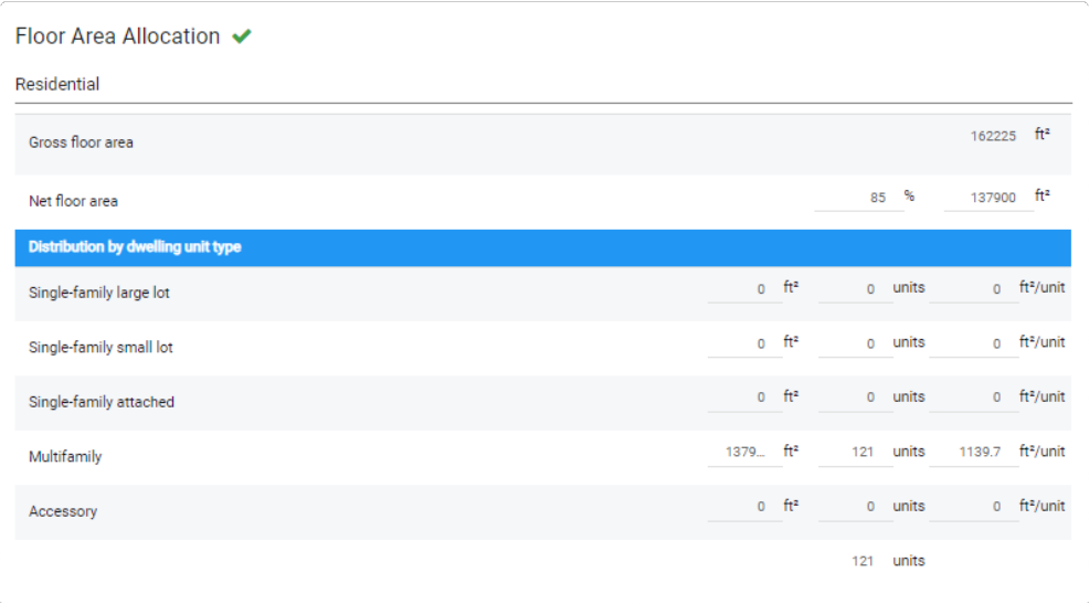
Residential section of the Floor Area Allocation panel
The residential allocations yield dwelling unit densities. Household and population densities are subsequently determined according to project-level variables for residential building occupancy and household sizes by dwelling unit type; see Use Library Settings for details.
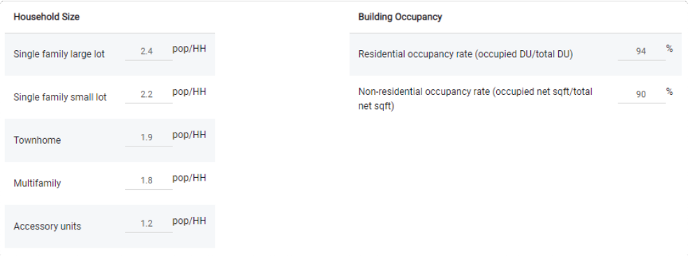
Variables for household sizes and building occupancy, accessed via Library Settings
Enter Non-Residential Floor Area Allocation details. The Non-Residential section of the Floor Area Allocation panel describes how non-residential building area is distributed among employment uses. Employment is represented by six top-level sectors and a number of sub-sectors that nest into them. Employment density is determined by the floor area allocations, along with assumptions for the distribution of employment by subsector, floor area per employee, and non-residential building occupancy. These assumptions are determined according to project-level employment variables and defaults; see Use Library Settings for details.
Gross floor area – The amount of gross floor area dedicated to non-residential uses. The value is set in the Building Characteristics panel and displayed here for reference.
Net floor area – Includes two values: a net floor area percentage and the resulting total net non-residential floor area in the building. Net, or leasable, floor area is calculated as the product of the net floor area percentage (also known as a net-to-gross ratio) and gross floor area.
Distribution by employment sector – Analyst quantifies the number of jobs accommodated by buildings according to specifications for how non-residential floor area is distributed, and variable assumptions for floor area per employee that are linked to the building density category specified in the Component Information panel. These specifications are required to support robust planning and analysis that account for employment by type, and the impacts of different uses on building energy use, water use, carbon emissions, and more.
Employment and associated building area are represented by six top-level sectors: Retail, Office, Public, Industrial, Agriculture, and Military. Inputs for each employment sector include gross floor area and the percentage of total gross floor area that it constitutes. For example, a building with ground-floor retail and four floors of office space above might be represented by a distribution of 20% Retail and 80% Office.
Each sector row contains a value for gross floor area and the percentage of floor area allocated to the sector. The area and percentage are tethered such that editing one automatically updates the other. The Edit button
 to the right of the percentage brings up a window to allow you to set the distribution of employment by subsector, which determines the number of employees accommodated by the specified floor area. The employment sectors and subsectors are listed below.
Retail – Includes Retail Services, Restaurant, Arts & Entertainment, Accommodation, and Other Services.
Office – Includes Office Services and Medical Services.
Public – Includes Public Administration and Education Services.
Industrial – Includes Manufacturing, Wholesale, Transportation & Warehousing, Construction, and Utilities.
Agriculture – Includes Agriculture and Extraction.
Military – Includes Military only.
Overallocated / Unallocated – A value that appears if the sum total of floor area by sector does not equal the total non-residential gross floor area, and the percentages do not add up to 100%. Use this value to correct the floor area allocations. The Component will not be valid for use if there is any overallocated or underallocated area.
For our example, we have entered the values below based on given development information.
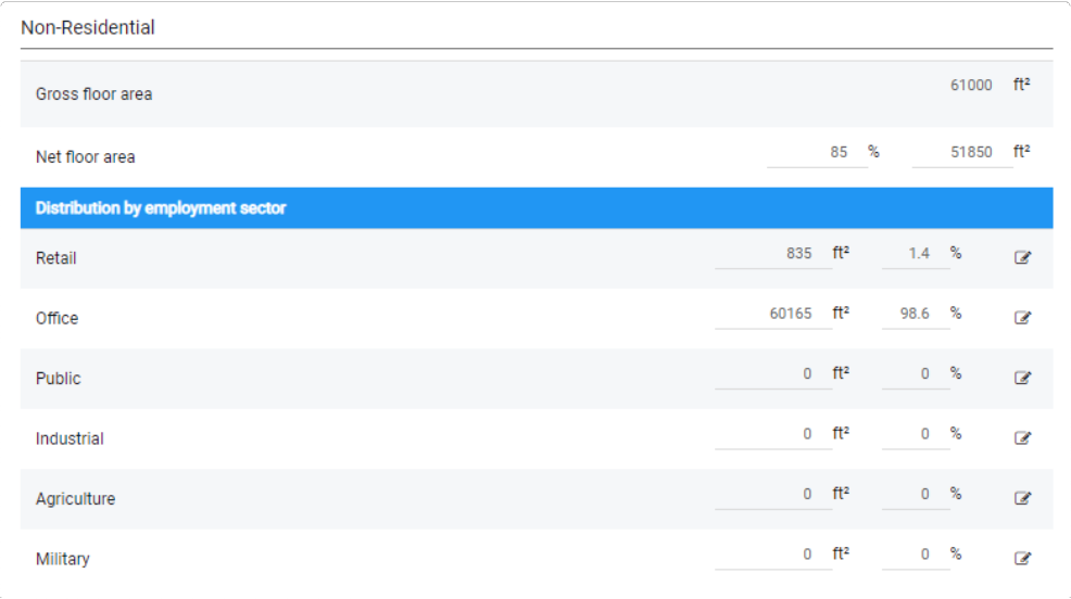
Non-Residential Floor Area Allocation for example building
Employment by Subsector – The subsector distributions are accessed via the Edit button
located to the right of the employment sector floor area percentage. Clicking the button opens the Employment by Subsector window for the selected sector.Subsector employment percentage – The percentage of jobs in each subsector is an input. The floor area by subsector is calculated based on the inputs and shown in the Area column at left. The assumed floor area per employee by subsector is shown in the column at right.
The Retail sector employment distribution for our example is shown below. The net area for an on-site restaurant was given, comprising the only retail use in the building.
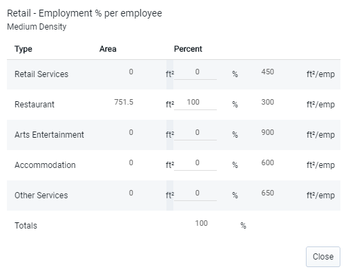
Retail sector employment distribution for example building
Upon Component creation, the model is seeded with a default distribution of employment by subsector as specified in Library Settings. The variable assumptions for floor area per employee by subsector are also specified there. The Employment Variables and Defaults section of the Library Settings screen is shown below. See Use Library Settings for details.
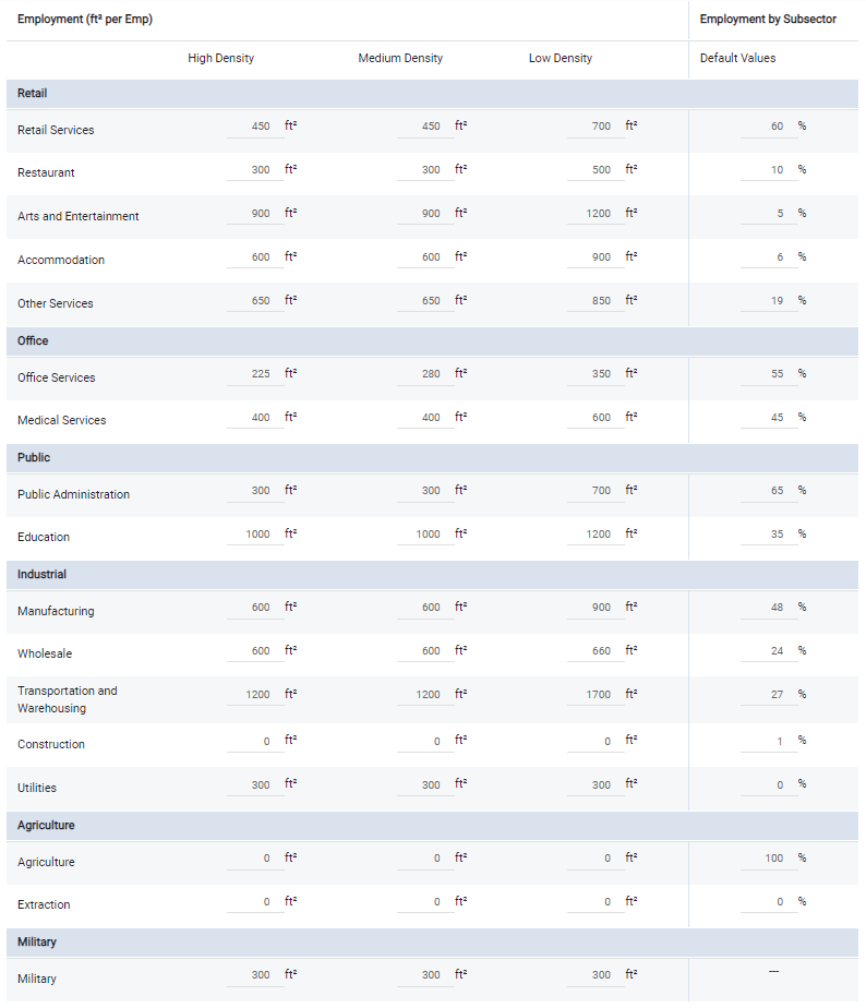
Library Settings for floor area per employee variables and employment distribution by subsector defaults
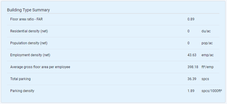
Review the summary information for your Component – The resulting characteristics of your Component, including floor area ratio (FAR); net residential, population, and employment densities; average gross area per employee; and parking density, are summarized in the Component Summary panel. The summary for our example building is shown below.
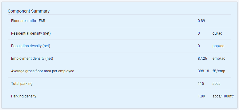
Component Summary for example building
Save your input – Click Save. Your Component will be saved. If the specifications are not valid, your Component will be saved but cannot be used in type definitions until the inputs are rectified.
Create a Building Type
Building Types are used to represent buildings, parks, and other elements in terms of their detailed built form characteristics. They are defined as a composite of one or more Components. While Building Types are used in painting scenarios, Components can only be used as ingredients for Building Types.
In the previous tutorial, we created a Component from scratch, and in so doing stepped through the detailed building and site characteristics that are the foundation for all Building and Place Types. In this tutorial, we'll create a new Building Type using the Land Use Type Manager, and view its resulting characteristics.
For more information about land use types, the Land Use Type Manager, and Library Settings, see the Land Use section of the Features documentation.
Data Layers | Features |
None |
You can add a new Building Type to your library in either of two ways: by creating it from scratch, or as a copy of an existing type that you then edit. For our example, we'll create two Building Type variations to demonstrate how Component characteristics are blended.
Enter Manage mode. Click the Manage icon
from the left-hand menu bar.From Manage mode, navigate to the Building Types screen.
Click the Add new button. A new Building Type window appears.
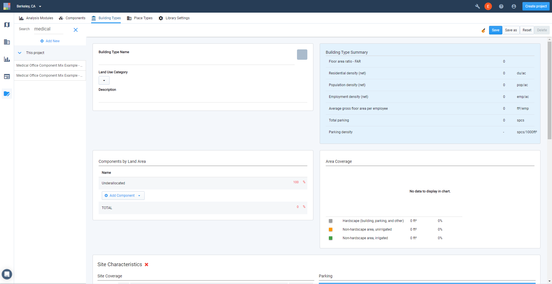
New Building Type window
Enter Building Type Information. The Building Type Information panel contains basic information for identifying and categorizing the Building Type.
Building Type Name – Names can be as descriptive as you like. If you're creating a number of local Building Types, it can be useful to add an identifier to their names so that you can easily filter your Building Types list using the search box.
Building Type Identifier – A colored square containing the initials of the Building Type name, used as quick identifier here and in the Build Scenario > Building Types menu. A default color is selected based on land use category. Click on the chip to change the color.
Land Use Category – Refers to the Land Use Category (L3) designation. Select the L3 category that the Building Type should be associated with. The L2 and L1 level designations are automatically designated on the basis of L3. (See Land Use Hierarchy for more information.)
Description – A description of the Place Type. This field is optional.
Place Types – This is a list of the Place Types in which the Building Type is included. The list is automatically generated. The Place Type names link to the Manage screen for the Place Types.
The inputs for our first example Building Type are shown below.
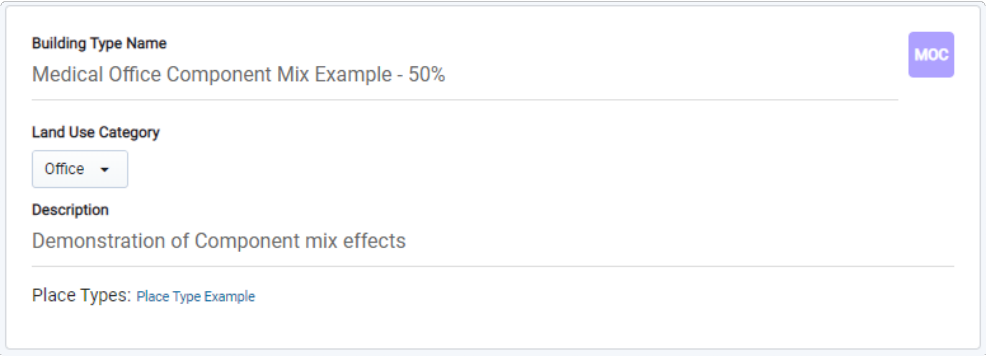
Building Type Information panel
Specify a Building Type to include 50% of a single Component. We're going to use the Component we created in the previous tutorial. We'll create two type variations: one that contains only the Medical Office Campus Component, and another that blends it with undeveloped land. The differences between the two should help reveal how the Component mix calculations work to result in building and density characteristics.
Click the + Add Component button in the Components by Land Area panel. A Component selection window appears.
Select a Component to add. You can type on the Search line to find the Components you want to add. For our example, we'll add the Medical Office Campus Component we created earlier. You may follow along using a different Component.
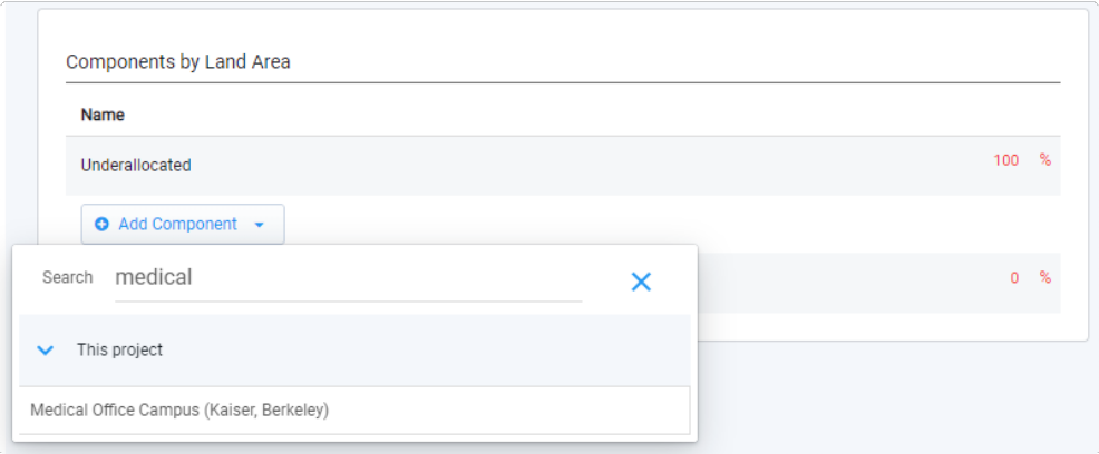
Component selection window
Specify a Component percentage. This is the share, in terms of land area, that the Component will account for in the Building Type. For our first Building Type, set the percentage to 50%.
Select another Component to add. This time, add the default Component called Blank Data. This Component contains only non-hardscape area, with no buildings—it is effectively empty.
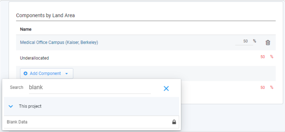
Component selection window
Set the Blank Data Component percentage to 50%. Now your Component percentages add up to 100%, and your Component is valid.
Click the Save button to save the Building Type.
Specify a second Building Type to include 100% of a single Component. To contrast with the first example, we'll create a second Building Type to include the Medical Office Campus Component at 100%.
Click the Save as button and enter a name for a second Building Type.
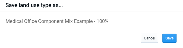
Save as window
Click the Delete button
 for the Blank Data Component in the Components by Land Area panel.
Adjust the Medical Office Campus Component percentage to 100%.
Click the Save button to save your second Component.
Review the characteristics of the "100%" Building Type comprised entirely of the example Component. Explore the values in the Area Coverage, Site Characteristics, Building Characteristics, and Floor Area Allocation panels to see how the original Component has been translated into a Building Type. (You can return to the Component screen to compare the Component inputs with the resulting Building Type characteristics.)
At the Building Type level, all building and site characteristics are normalized to one acre. Building and site area are expressed as percentage distributions by category. Dwelling units are expressed in densities per acre rather than counts. Finally, the non-residential floor area distributions are translated into employment densities per acre, by sector.
The summary characteristics of the Building Type, including FAR and densities, are the same as for the original Component. In cases where you want to be specific in defining building characteristics, it may be useful to you to create single Components for application as Building Types.
Compare the characteristics of the 100% Building Type with the 50% Building Type. Now we'll compare the results of our two Building Type variations. The summary panels are shown below. Note that the building characteristics—FAR, gross floor area per employee, and parking density—remain the same. The Building Type mix consisted of one building only, and its characteristics did not change.
However, the density characteristics of the two Building Types differ. As you might expect, the Building Type that blends the Component with an equal percentage of undeveloped land has an employment density that is half that of the full-strength Component.
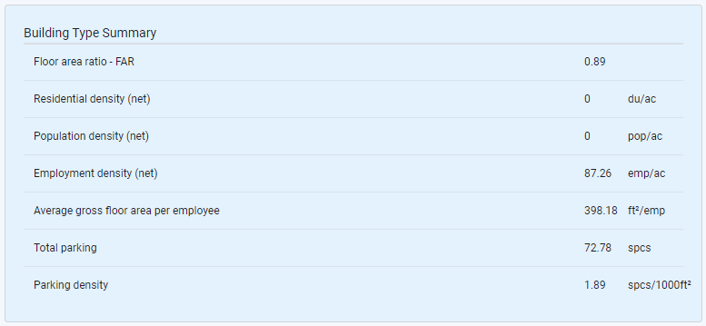
Summary for the Building Type that includes 100% of the example Component
Summary for the Building Type that includes 50% of the example Component, and 50% undeveloped land
Create a Place Type
Place Types represent places—combinations of different types of buildings and the streets, parks, and other elements of urban infrastructure that surround them. A Place Type can be used to represent, for example, the mixed-use center of a town, or development along an auto-oriented suburban retail corridor. In technical terms, they encompass both "net" parcel area occupied by Building Types and "gross" area occupied by rights-of-way.
Place Types are defined as composites of one or more Building Types. In the previous tutorial, we created a Building Type comprised of a single Component. In this tutorial, we'll use that Building Type to create a new Place Type, and view its resulting characteristics.
For more information about land use types, the Land Use Type Manager, and Library Settings, see the Land Use section of the Features documentation.
Data Layers | Features |
None |
You can add a new Place Type to your library in either of two ways: by creating it from scratch, or as a copy of an existing type that you then edit. For our example, we'll create a Place Type that blends the Medical Office Building Type that we created with Analyst default Building Types to represent mixed development on a block.
Enter Manage mode. Click the Manage icon
 from the left-hand menu bar.
From Manage mode, navigate to the Place Types screen.
Click the Add new button. A new Place Type window appears.
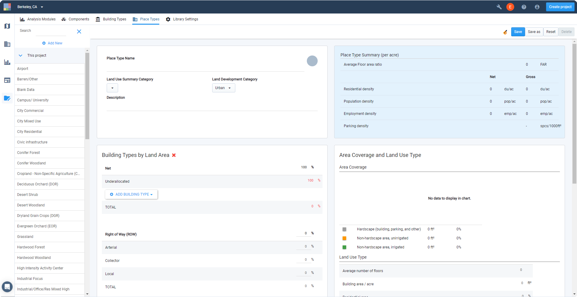
New Place Type window
Enter Place Type Information – The Building Type Information panel contains basic information for identifying and categorizing the Building Type.
Place Type Name – Names can be as descriptive as you like. If you're creating a number of local Place Types, it can be useful to add an identifier to their names so that you can easily filter your Place Types list using the search box.
Place Type Identifier – A colored circle containing the initials of the Place Type name, used as quick identifier here and in the Build Scenario > Place Types menu. A default color is selected based on land use category. Click on the chip to change the color.
Land Use Summary Category – Refers to the Land Use Summary (L1) designation. Select the L1 category that the Place Type should be associated with. (See Land Use Hierarchy for more information.)
Description – A description of the Place Type. This field is optional.
The inputs for our example Place Type are shown below.
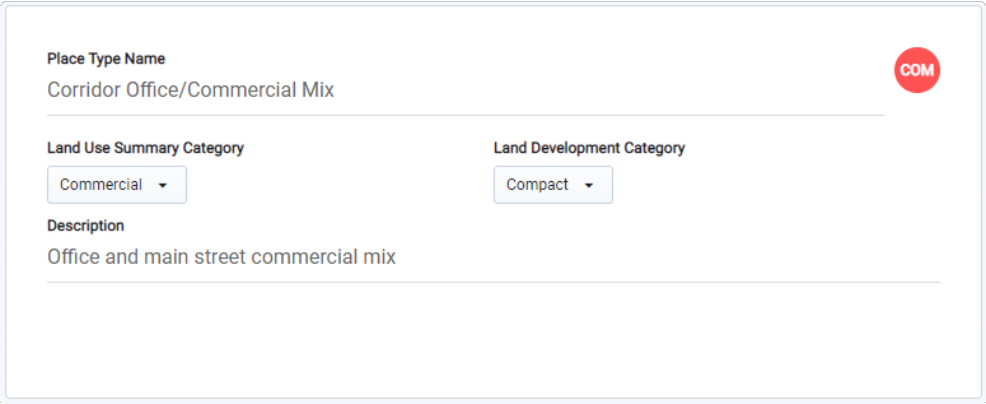
Place Type Information panel
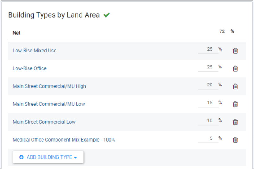
Add Building Types. We'll use the Medical Office Building Type we created in the previous tutorial, along with some others from the default library.
Click the + Add Building Type button in the Building Types by Land Area panel. A Building Type selection window appears.
Select Building Types to add. You can type on the Search line to find the Building Types you want to add.
Specify Building Type percentages. The percentages represent the share, in terms of land area, that each Building Type will account for in the Place Type. For our example, we'll mix Building Types as shown below.
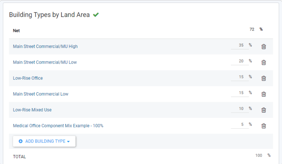
Sample Building Type mix
Specify the Right of Way (ROW) percentage. For our example, we'll assume that right-of-way area accounts for approximately 28% of gross area. Note that the net area is automatically calculated to account for 72% of gross area.
Specify ROW area distribution. We'll assume a right-of-way area distribution of 65% arterial, 10% collector, and 25% local roadways.
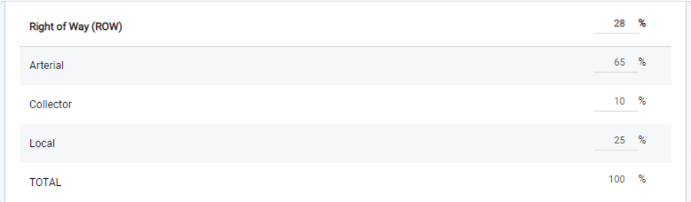
Right of Way allocations
Save the Place Type. Click the Save button.
Review the characteristics of the resulting Place Type. Explore the values in the Area Coverage, Site Characteristics, Building Characteristics, and Floor Area Allocation panels. Note the average floor area ratio (FAR) and differences between the net and gross densities as shown in the Place Type Summary.
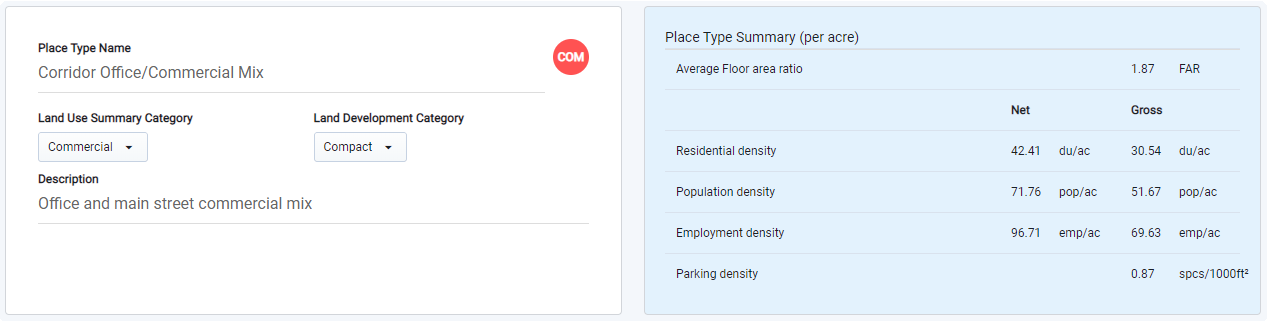
Place Type Information and Summary
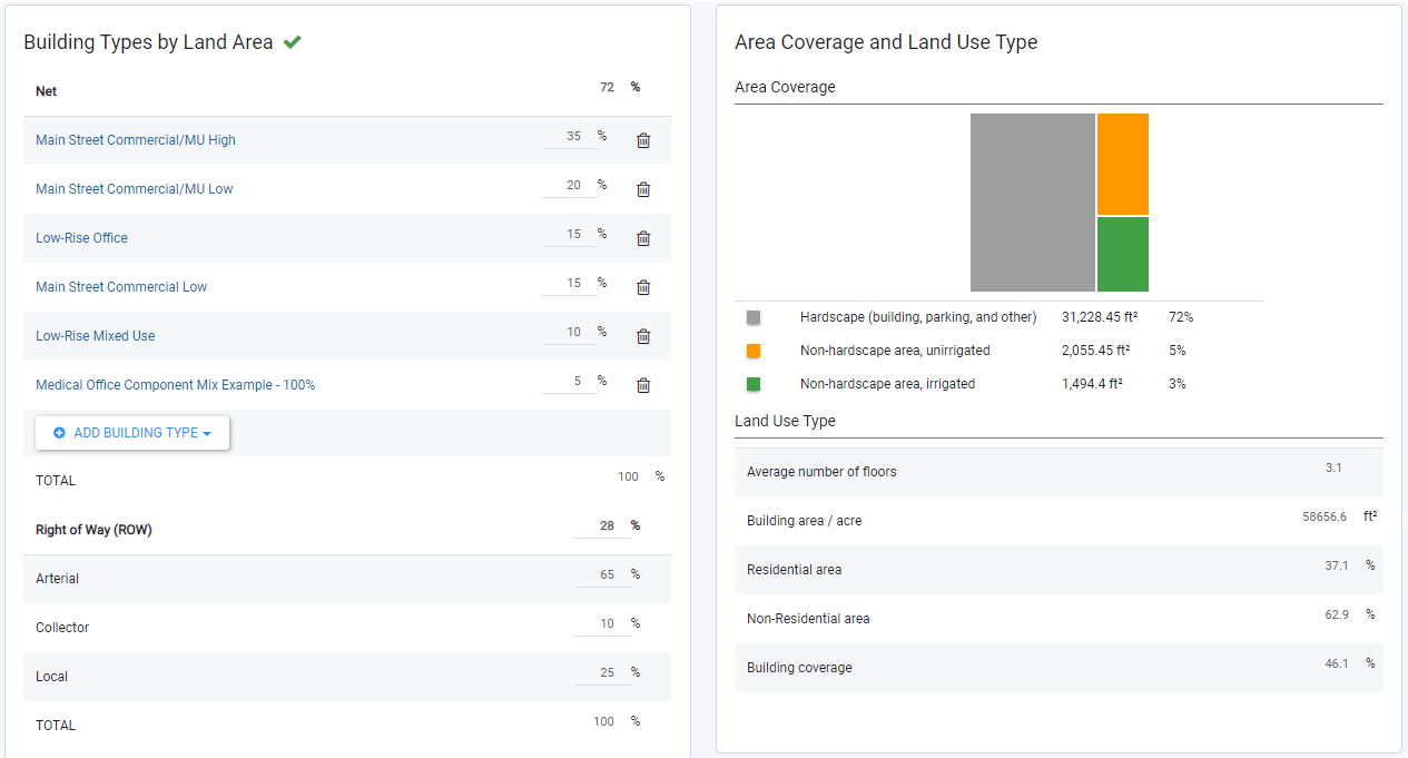
Building Type mix and Area Coverage
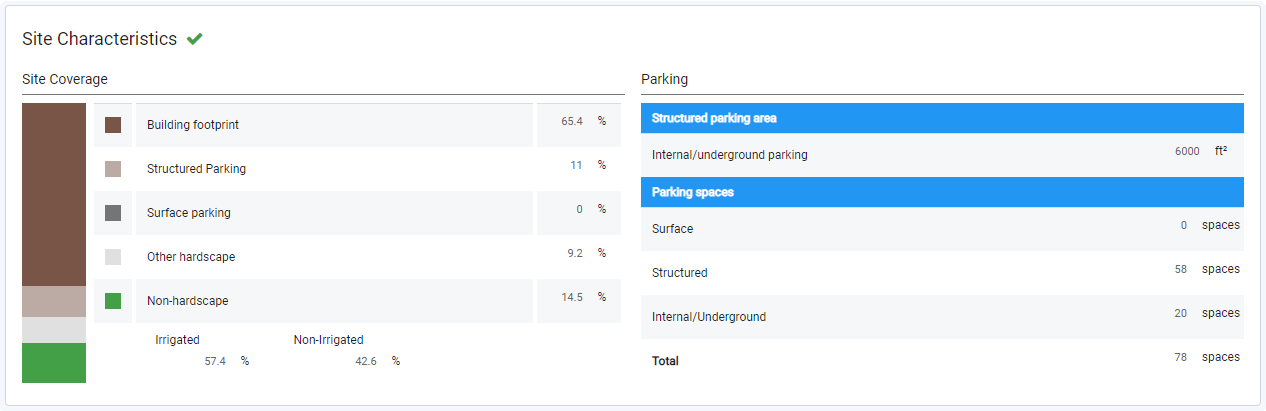
Site Characteristics
Building Characteristics
Residential and Non-Residential distributions
Tune the characteristics of the Place Type. For our example, we'll assume that with this Corridor Office/Commercial Mix type we want to reach an average 2.0 FAR. The current FAR is 1.87. What kind of development meets that higher target?
Adjust the Building Type mix. We'll keep the same set of Building Types, but change the distribution to include a higher proportion of the Low-Rise Mixed Use type, which has the highest FAR among the included types.
Revised Building Type mix
Review the resulting Place Type characteristics. The revised mix of buildings has increased the residential and employment densities, and the distribution of employment among the Retail and Office sectors, as shown in the residential and non-residential building details.

Revised Residential and Non-Residential distributions
The Place Type Summary shows the new FAR and densities.
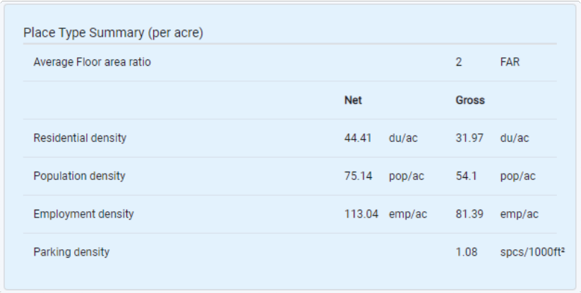 |
New Place Type Summary
You can make adjustments to your Place Types by iterating on the Building Type mix or, if necessary, revisiting your Building Types to ensure that are representative of potential development in your project area.
Scenario Painting by Type
Land use scenarios are built by applying population, housing, employment, and development attributes to the parcels or blocks that comprise a scenario canvas. These attributes can be applied by "painting" canvas features with land use types (Building Types or Place Types). As a complement to painting by type, you can also paint "by attribute" to directly specify values for dwelling units, employment, and their associated building area. In this tutorial, we'll create a new scenario and get started with painting by type. In the next tutorial, we'll focus on painting by attribute.
Before you start developing scenarios, it's important to review the land use types and library settings that you will be using. You may use the default set of types that come loaded with Analyst, or you may choose to create your own. See the previous tutorials on creating Components and types for guidance.
Data Layers | Features |
Scenario Canvas |
Create a new scenario. Click the
 icon to the right of the scenario tabs and select the Base Scenario or any existing scenario as the basis for your new scenario.
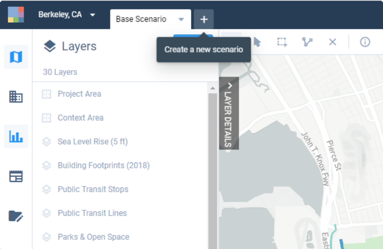
Creating a new scenario
Alternatively, click to expand the menu for either the Base Scenario tab or the tab of the existing scenario you would like to copy. Select Create scenario (if creating a scenario from the Base Canvas) or Duplicate (if creating a scenario as a copy).
Your new scenario will be created and a tab for your new scenario will appear when finished. You'll also see a confirmation message at the bottom of your screen.
Whether created as a clone of the Base Canvas or as a duplicate of an existing scenario, your new scenario will maintain all the data layers of the original scenario, with the exception of any analysis output layers. Analysis output layers are generated the first time you run a module for a scenario.
Rename your new scenario. By default, new scenarios are given names with sequential numbers. Click to expand the menu for the tab of your new scenario, then select Edit Details. Enter a scenario name and description in the window that appears.
Activate the Scenario Canvas layer for your new scenario. The Scenario Canvas represents your scenario. When you create a new scenario from the Base Scenario, the Scenario Canvas is created as a copy of the Base Canvas.
Symbolize the Scenario Canvas layer on the 'Land Use Type (L4)' column. This column contains the Building and/or Place Type classifications for the Base Canvas.
Enter Build mode. Click the Build iconin the Mode bar. Alternatively, you can enter Build mode by activating the Scenario Canvas layer and selecting the Build tab in the Layer Details pane. The Build controls appear in the Layer Details pane.
Select one or more features on the Scenario Canvas to paint. You can select features using the manual selection tools, or apply filters to select features based on particular criteria—for example, vacant parcels, parcels within a size range, parcels within walking distance of transit, or underutilized parcels suitable for redevelopment.
You can also use reference data layers, or upload local data, to use as join layers to create filtered selections of features in the Scenario Canvas. In this manner, you could use data representing zoning, land use plans, or planned development projects as guides to select and paint features.
For our example, we'll apply a filter to select features according to their existing Building Type.
Click the Filter tab for the Scenario Canvas.
Click Add filter +, then select the Land Use Type (L4) column.
Select Parking Surface Lot from the list of L4 values. (Since our project uses a parcel-level canvas, the L4 values are Building Types.)
Click the Zoom to selection
 map view control to see the extent of where the selected features are located.
Pan and zoom on the map to review the selection of features. Using the Satellite base map option and decreasing the opacity of the scenario canvas can help with a visual review.
Edit your selection. You may choose to refine your filter criteria—for example, to filter by feature size using the Gross Area column. You can also edit your selection manually by holding down the Shift key and using the Point selection tool
 to deselect features. (You cannot add features to your selection if they do not meet the filter criteria that you already specified.)
Our filter resulted in a selection of 56 parcels. Though in reality we wouldn't paint them all with the same type, we'll keep our sample selection simple and not edit it any further.
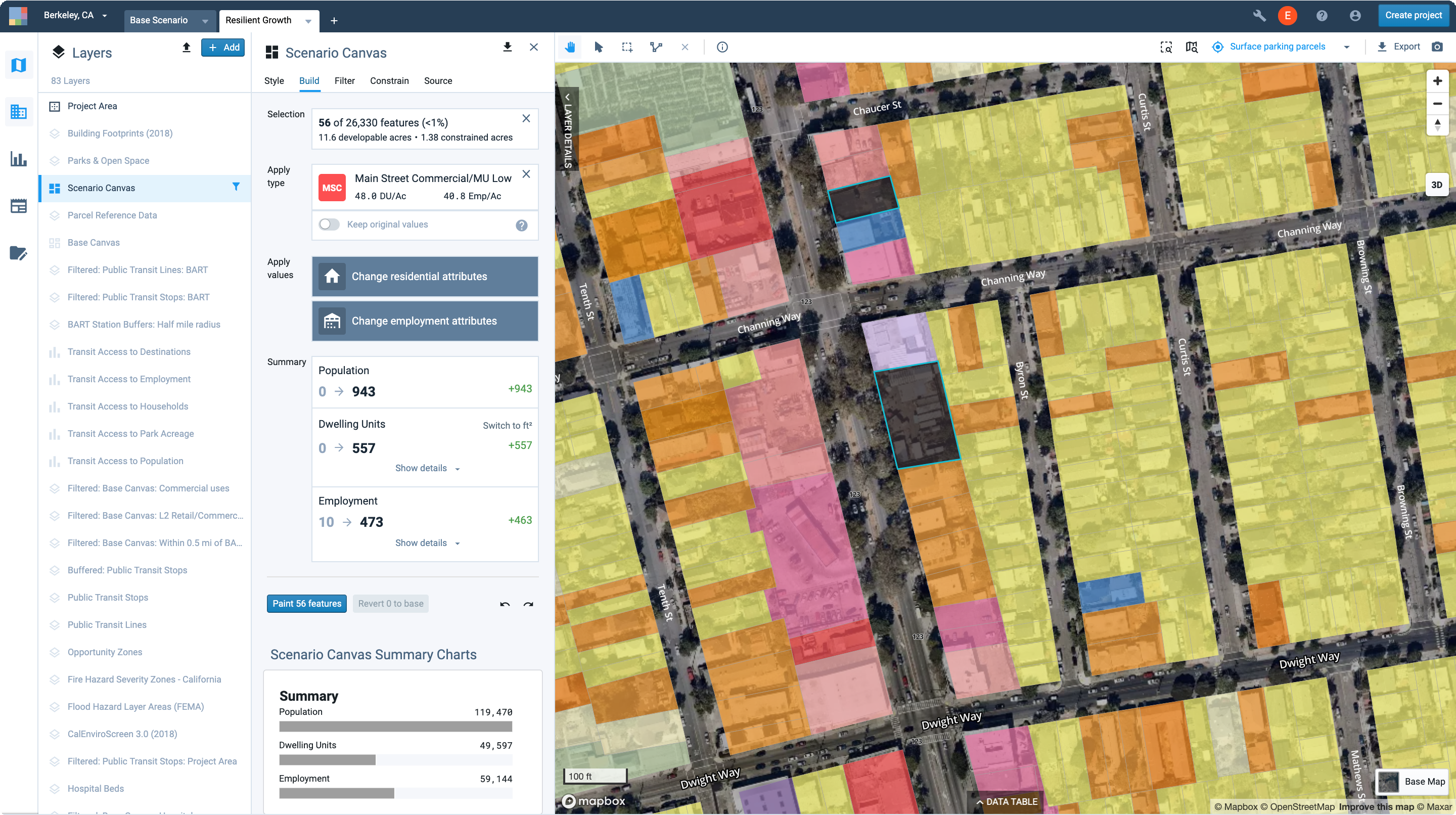
Scenario Build mode, with a map view showing two of the selected features to be painted
Select a type to paint with. Click the Building Types button to open the Building Types selection window. The menu entry for each type indicates the residential and employment densities. You can click the expand arrow in the upper right corner to see more details. Select a type and the window will close.
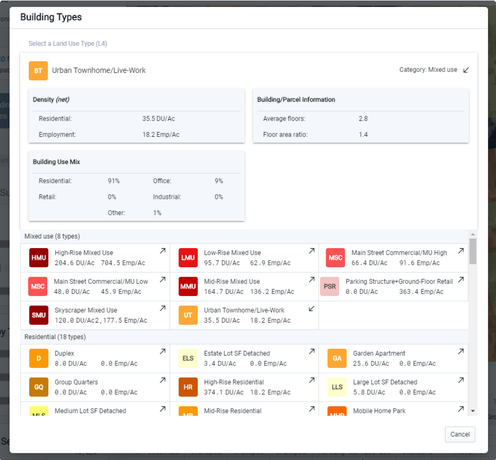
Building Types selection window
Review the program summary corresponding to your selection. The summary contains dwelling unit (DU), population, and employment counts associated with the selected features and type to be painted. You can use this information to decide whether to paint or change your selections.
The program preview for the paint selection shows that painting the 56 parking lot parcels with the "Urban Townhome/Live-Work" Building Type will accommodate 557 new dwelling units, 943 residents, and 473 new employees. The 10 employees associated with development in the Base Canvas will be lost.
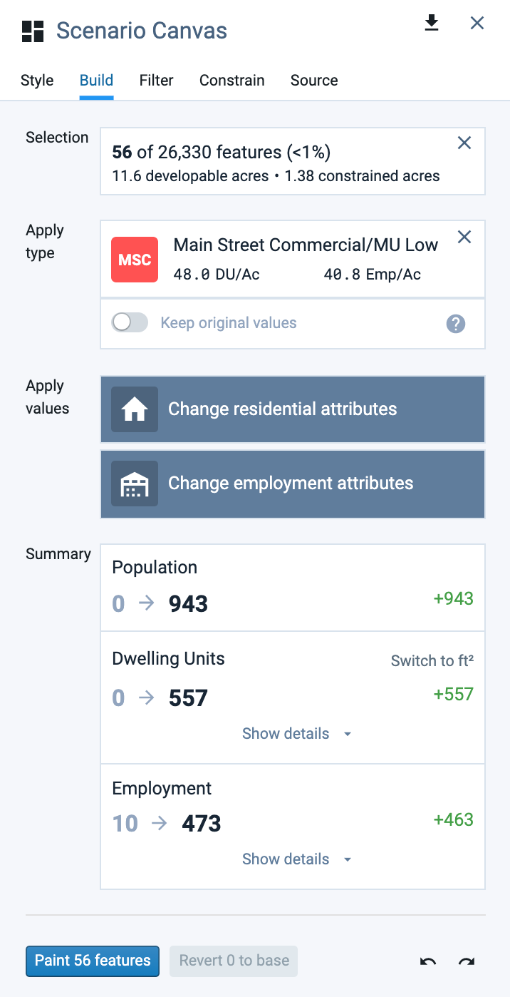
Program summary of attributes to be painted
Apply the selected type. Click the Paint 56 features button. The features will be painted accordingly. The paint will be reflected in the Painted row of the Program table, in the scenario canvas summary charts, on the map, and in the Data Table.
Reverse your paints. If you need to make any changes, use the Revert x to base, Undo
, or Redo controls. Reverting effectively returns features to their base condition. Undo and redo are applied to your sequence of past actions, independent of the features that are currently selected.Track scenario growth. As you continue to select and paint features, use the scenario canvas summary charts to track scenario growth. The charts are especially useful if you're building scenarios to meet control totals for new growth.
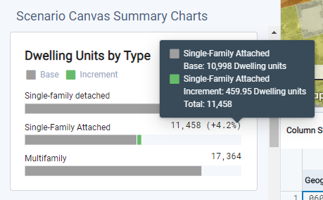
The Dwelling Units by Type summary chart tracks scenario growth
View comparative statistics for your scenario. Enter Report mode and select Summary Statistics to see charts that compare population, housing, households, jobs, and building area characteristics across scenarios.
Scenario Painting by Attribute
Create a new scenario, paint dwelling units and employment, and track growth.
Land use scenarios are built by applying population, housing, employment, and development attributes to the parcels or blocks that comprise a scenario canvas. Painting "by type" applies these attributes according to the densities of Building Types or Place Types. Painting "by attribute" allows you to depart from land use type densities and directly specify values for dwelling units, employment, and their associated building area. In the previous tutorial, we learned how to paint by type. In this tutorial, we'll focus on painting by attribute.
Data Layers | Scenario Canvas |
Features |
To start, set up a scenario and enter Build mode. From there, we'll step through a few examples of painting by attribute to meet different needs, including painting a planned project and painting single-family development.
Enter Build Mode
Create a new scenario. Click the
 icon to the right of the scenario tabs and select the Base Scenario or any existing scenario as the basis for your new scenario.
Creating a new scenario
Alternatively, click to expand the menu for either the Base Scenario tab or the tab of the existing scenario you would like to copy. Select Create scenario (if creating a scenario from the Base Canvas) or Duplicate (if creating a scenario as a copy).
Your new scenario will be created and a tab for your new scenario will appear when finished. You'll also see a confirmation message at the bottom of your screen.
Whether created as a clone of the Base Canvas or as a duplicate of an existing scenario, your new scenario will maintain all the data layers of the original scenario, with the exception of any analysis output layers. Analysis output layers are generated the first time you run a module for a scenario.
Rename your new scenario. By default, new scenarios are given names with sequential numbers. Click to expand the menu for the tab of your new scenario, then select Edit Details. Enter a scenario name and description in the window that appears.
Activate the Scenario Canvas layer for your new scenario. The Scenario Canvas represents your scenario. When you create a new scenario from the Base Scenario, the Scenario Canvas is created as a copy of the Base Canvas.
Symbolize the Scenario Canvas layer on the Land Use Type (L4) column. This column contains the Building and/or Place Type classifications for the Base Canvas.
Enter Build mode. Click the Build icon
 in the Mode bar. Alternatively, you can enter Build mode by activating the Scenario Canvas layer and selecting the Build tab in the Layer Details pane. The Build controls appear in the Layer Details pane. You're now ready to follow along with any of the examples below.
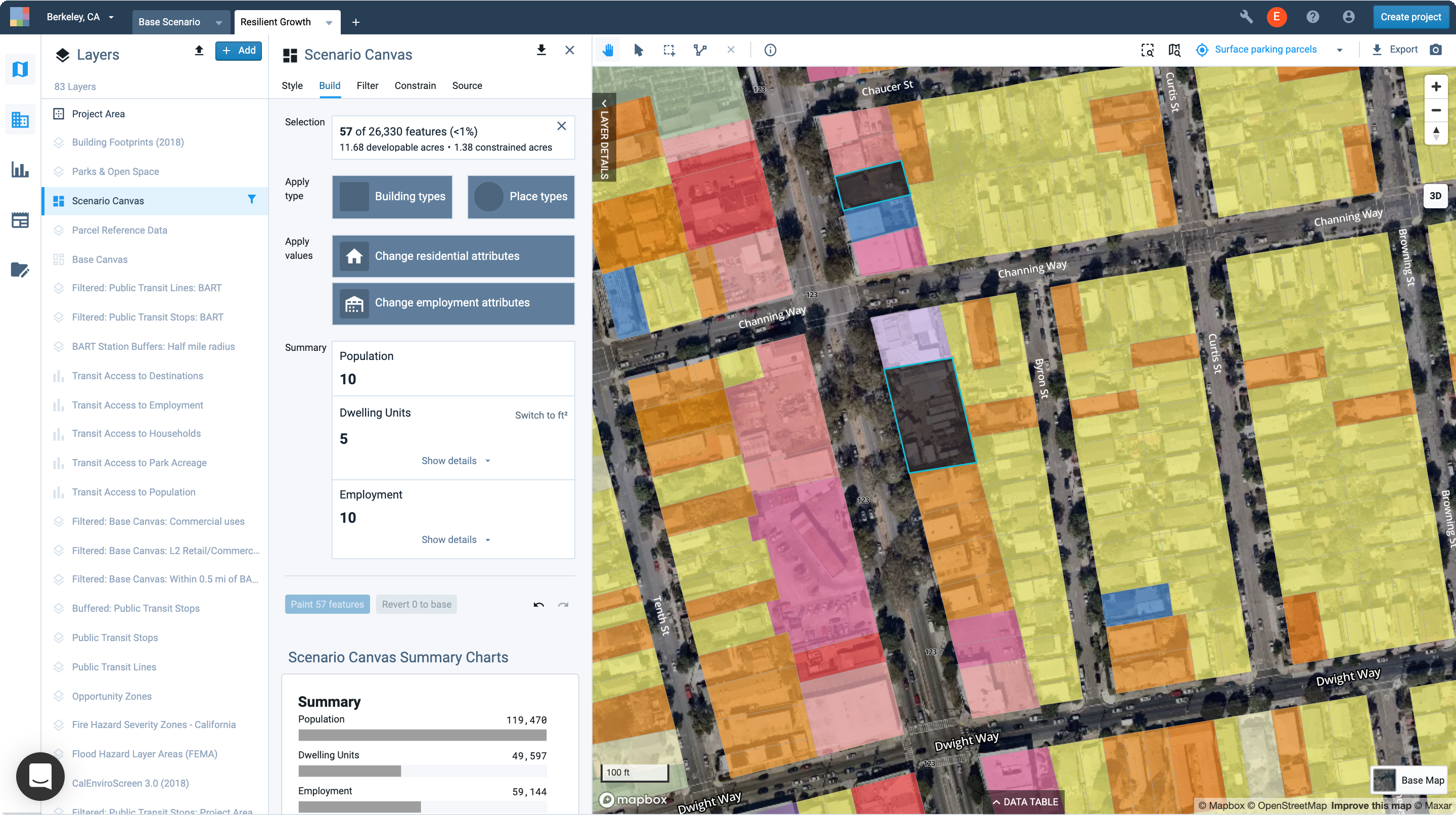
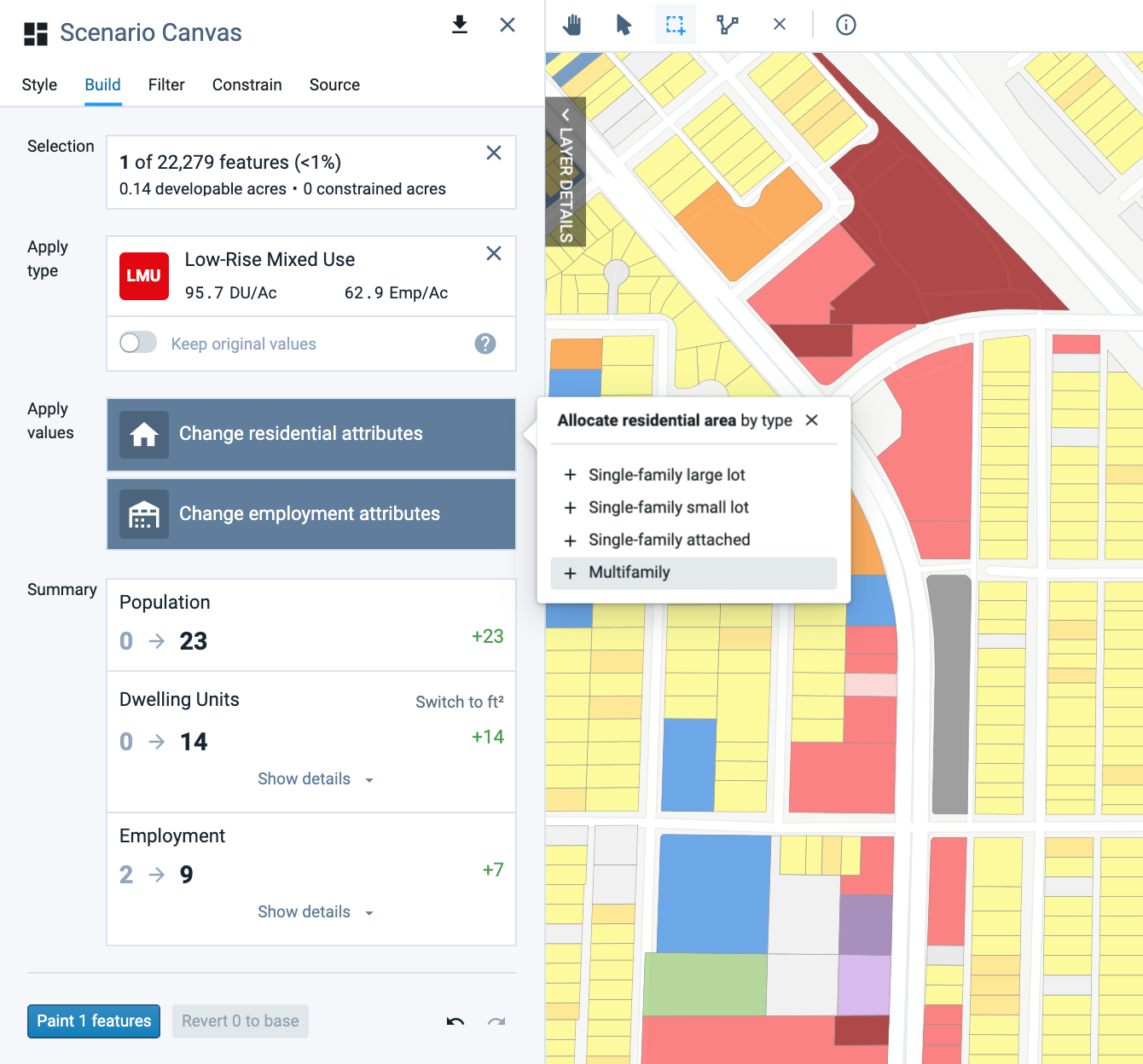
Scenario building controls
Paint a Planned Project
In this example, we'll paint a parcel to represent given information about a planned project. Painting by attribute allows you to quickly apply new dwelling units and employment without entering Manage mode and creating a representative land use type. Creating a new type, on the other hand, would be more appropriate for specifying detailed development characteristics, such as site coverage, or replicating the same development program at a later time.
Select a parcel on the Scenario Canvas to paint. Pan and zoom to a parcel and select it using the pointer tool. While you can paint multiple features at once, for this example we'll work with a single parcel.
Select a Building Type representative of the planned development. In this case, the selected type will be applied in name only since we'll go on to manually specify the residential and employment attributes to be painted. Selecting a type will set the L1 to L4 land use categories of the feature, which are important for mapping and working with a scenario.
Click the Building Types button to open the Building Types selection window. The menu entry for each type indicates the residential and employment densities. You can click the expand arrow in the upper right corner to see more details. Select the Mid-Rise Mixed Use type and the window will close.
Building Types selection window
See the program summary corresponding to your selection. The Summary section shows the population, dwelling unit (DU), and employment counts for the base, followed by the counts that would result if the parcel were painted with the selected type. The net growth or loss between the base and future scenario allocation is also shown.
The program preview for our selection shows that painting the selected parcel with the Mid-Rise Mixed Use type would result in 83 residents, 49 dwelling units, and 40 employees.
Program summary for the paint selection
As you change the residential and/or employment area attributes in the steps that follow, the program summary will change. You can expand the view to see dwelling units by type and employment by sector by clicking Show details.
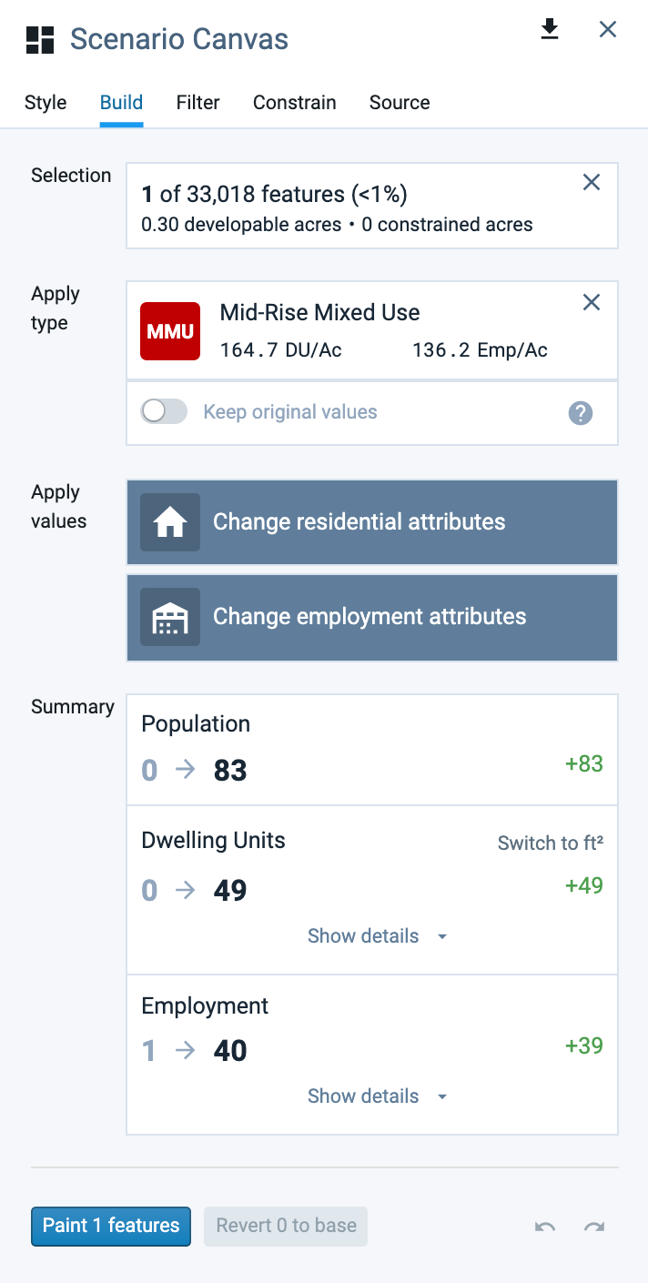
Click the Change residential attributes button. We'll first enter information about the residential portion of the planned mixed-use development. A menu of housing types will appear.
Selecting a housing type to add
Select the Multifamily housing type. The Allocate residential area by type window will appear with an entry row for multifamily units.
Select Apply per feature from the drop-down menu. We'll specify a number of dwelling units to be painted on the parcel. When multiple canvas features are selected, “Apply per feature” paints the same number of units on each, regardless of land area. “Apply per acre” paints units by density on the developable land area of the selected features.
Enter a number of units and unit size. Enter 28 units at 845 net square feet each. The total floor area associated with your entries, in this case 23,660 square feet, is shown to the right.
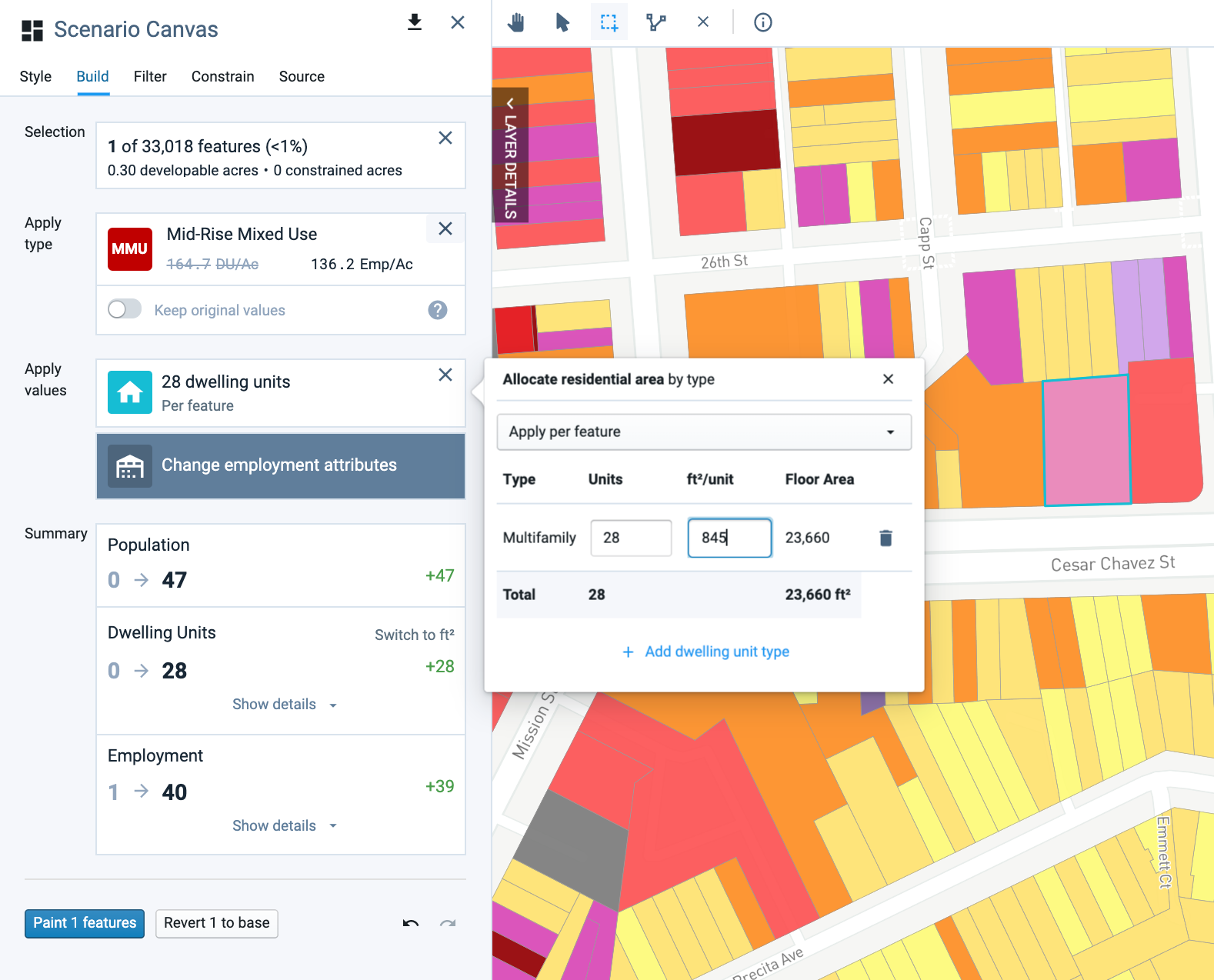
Entering residential attributes
The Summary section will be updated to show the 28 dwelling units entered so far, and their associated population. Population is calculated using the project-wide variables for the average multifamily household size and overall residential occupancy. These variables are set on the Library Settings page in Manage mode. Population cannot be edited independent of dwelling units for individual features.
Also notice that the density indicator in the land use type card gets crossed out to indicate that the original residential density for the type no longer applies. Since we haven't yet changed the employment attributes, the original employment density of the Mid-Rise Mixed Use type still applies.
Click the + Add dwelling unit type button and select Multifamily to add another entry row. You can add rows for other types of dwelling units, or for units of the same type with different sizes. For our example, we'll create multiple multifamily entries to reflect a mix of one- and two-bedroom apartments with average sizes of 845 and 1,150 net square feet, respectively.
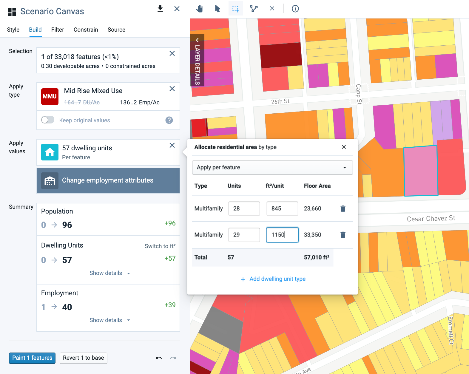
Creating multiple entries for different unit sizes
Entries are automatically saved; to remove an entry row, click the Delete icon
.Click the X button at the top right of the Allocate residential area by type window to close it.
Click the Change employment attributes button. Now, we'll enter information about the employment area of the planned development. A menu of employment sectors will appear.
Select the Retail employment sector. The Allocate employment area by sector window will appear with an entry row for Retail employment.
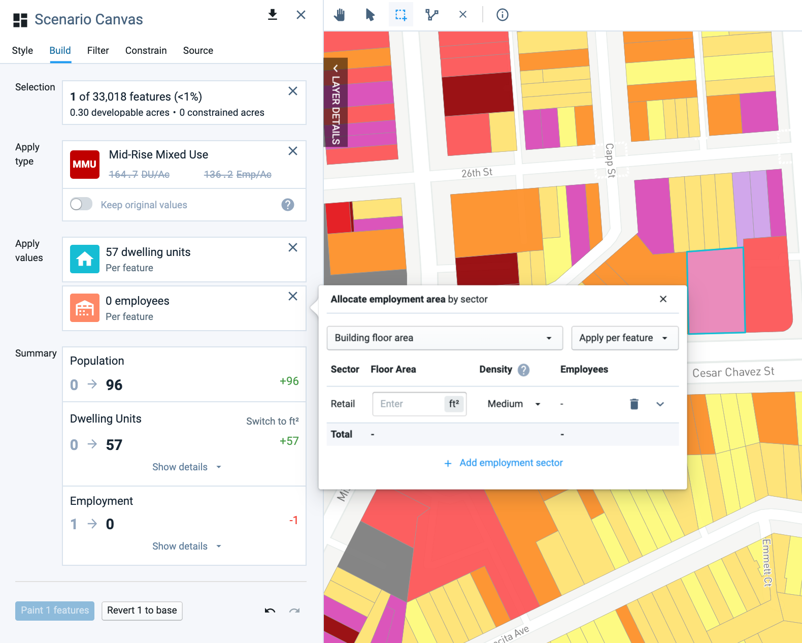
Allocate employment area by sector window
Select the Building floor area from the drop-down menu. You can enter employment information based on gross building floor area or numbers of employees. We'll enter floor area information since we have information about the planned retail and office space of the building.
Select Apply per feature from the drop-down menu. When multiple canvas features are selected, Apply per feature paints the same amount of building floor area and number of employees on each, regardless of land area. Apply per acre paints floor area and employees by density on the developable land area of the selected features.
Enter an amount of planned Retail building floor area. Enter 1,300 gross square feet. The corresponding number of employees will be shown to the right. The relationship between floor area and employees by sector is determined by an underlying distribution of employees by subsector, and variable assumptions for gross floor area per employee. We'll see these values soon.
Select the Medium building density category from the Density drop-down menu. The Low, Medium, and High building density categories are the same as those used in creating Components. Each category is associated with a different set of variables for floor area per employee, by subsector. These variables are set on the Library Settings page in Manage mode.
Click the Expand icon
 at the right end of the entry row. The distribution of Retail employees and building floor area by subsector will be shown, along with variable values for square feet per employee. In our example, we have a 50/50 distribution of employees between the Restaurant and Retail services subsectors, and an allocation of 500 square feet and 800 square feet of gross floor area for each, respectively.
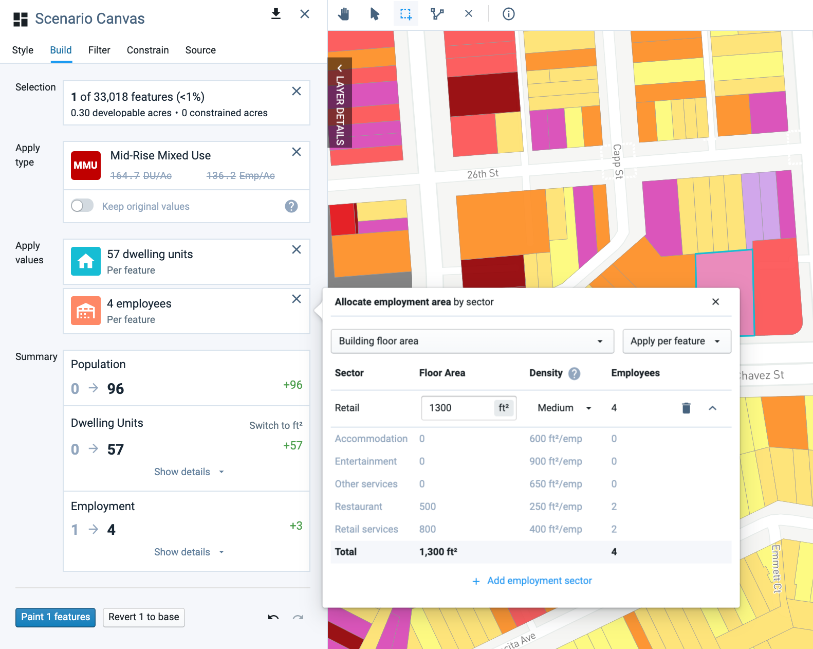
Viewing employment attributes by subsector
The distribution of employees by subsector is based on the default values set on the Library Settings page in Manage mode. While you cannot change the subsector employment distribution through the painting dialog, you can set the defaults in Library Settings prior to painting to populate the dialog with the intended values. The subsector distributions are static defaults, not variables, so changing them will not affect other painted features or land use types.
From the Library Settings page, you can also set the variables for gross floor area per employee. Variables are dynamic, so any changes to them affect all associated land use types, painting actions, and edits to the Base Canvas that involve changing employment values. The variables do not apply, however, to the base employment or building area values of unedited or unpainted features. See Use Library Settings for details on setting the variable values.
Once you specify new employment information, the Summary section will be updated to show the employment and building floor area associated with your entries. Also notice that the density indicator in the land use type card gets crossed out to indicate that the original employment density for the land use type no longer applies.
Click the + Add employment sector button and select the Office employment sector. We'll specify Office building area next. Enter 1700 square feet for the Office sector, again using the Medium building density category.
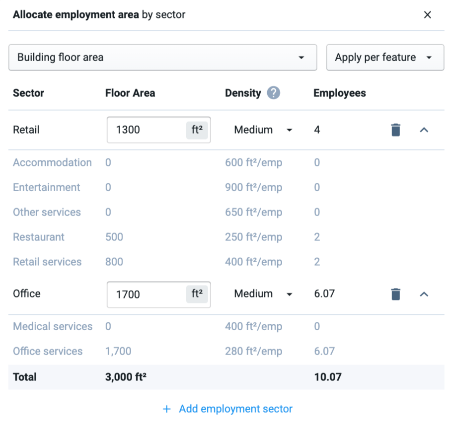
Entering attributes for multiple employment sectors
Entries are automatically saved; if you need to remove an entry row, click the Delete icon
.Click the X button at the top right of the Allocate employment area by type window to close it.
Review the program summary corresponding to your attribute entries. The summary contains population, dwelling unit (DU), and employment counts for the base, followed by the counts to be painted. The net growth or loss between the base and future scenario allocation is also shown. To see dwelling units by type or employment by sector, click the Show details buttons.
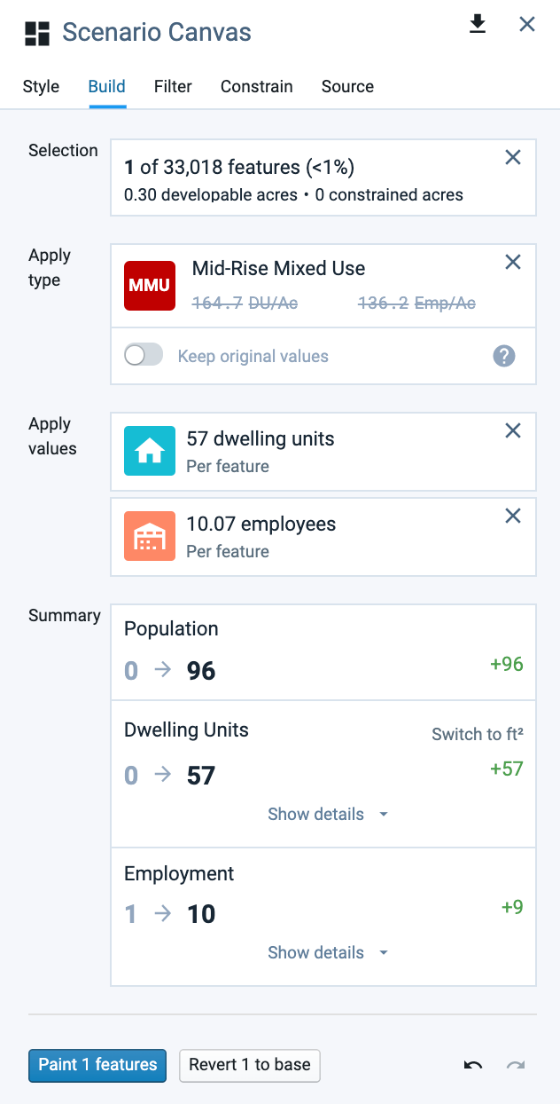
Program summary of attributes to be painted
Click the Paint x features button. The feature will be painted accordingly, and reflected in the scenario canvas summary charts, on the map, and in the data table for the scenario.
Paint Single Family Development
In this example, we'll paint single family detached residential development so that each parcel receives a single dwelling unit. Painting by type typically results in fractional numbers of units on individual parcels because, while lot sizes vary, Building Types have fixed densities. Painting units directly onto parcels allows you to be more precise in your allocations.
Select parcels on the Scenario Canvas to paint. For our example, we'll use filters on the scenario canvas to select vacant residential parcels that we'll paint with infill development.
Click the Filter tab for the Scenario Canvas.
Click Add filter +, then select the Land Use Type (L4) column.
Select Vacant Residential Lot from the list of L4 values.
Click Add filter +, then select the Gross Area column.
Enter a value range of 0.033 to 0.07 acres (approximately 1,450 to 3,000 square feet).
Review your selection using the map and data table, and make edits as needed. Our filters resulted in a selection of 41 parcels dispersed throughout residential neighborhoods in our project area.
Select a Building Type to assign to the painted parcels. Click the Building Types button to open the Building Types selection window, then select the Very Small Lot SF Detached type. The vacant parcels we selected fall within the lot size range of this type.
See the program summary corresponding to your selection. The summary shows the population, dwelling unit (DU), and employment counts for the base, followed by the counts that would result if the parcel were painted with the selected type. The net growth or loss between the base and future scenario allocation is also shown.
The program preview for the paint selection shows that painting the selected parcels with the Very Small Lot SF Detached type would result in 28 total dwelling units, as compared to the 41 units that there would be with a single unit on each parcel.
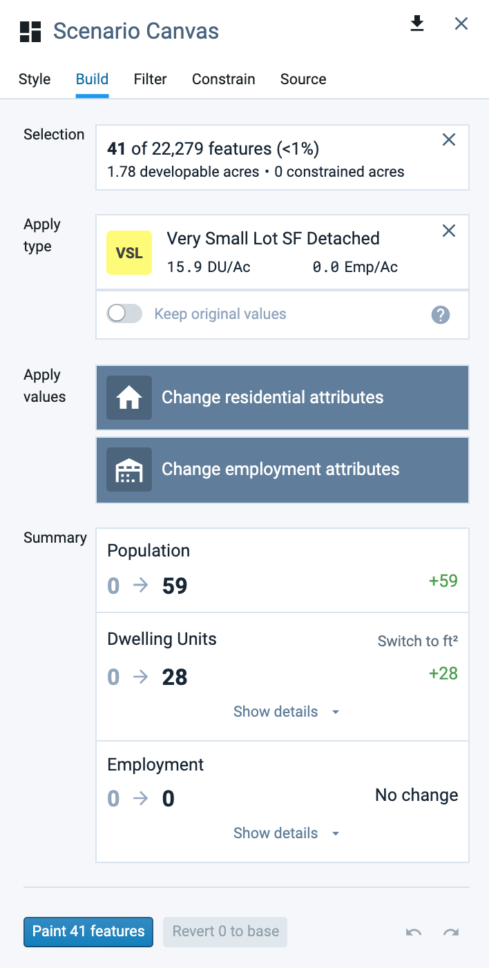
Program summary for painting with a selected type
As you change the residential attributes in the steps that follow, the program summary will change.
Click the Change residential attributes button. A menu of housing types will appear.
Select the Single-family small lot housing type. The Allocate residential area by type window will appear with an entry row for single-family small lot units.
Select Apply per feature from the drop-down menu. We'll specify a number of dwelling units to be painted on each parcel.
Enter a number of units and unit size. Enter 1 unit with a size of 1,200 square feet. This will paint the same average unit size on each parcel in the selection. (If you wanted to more closely match unit sizes to lot sizes, you could apply filters and paint using narrower parcel size ranges.)
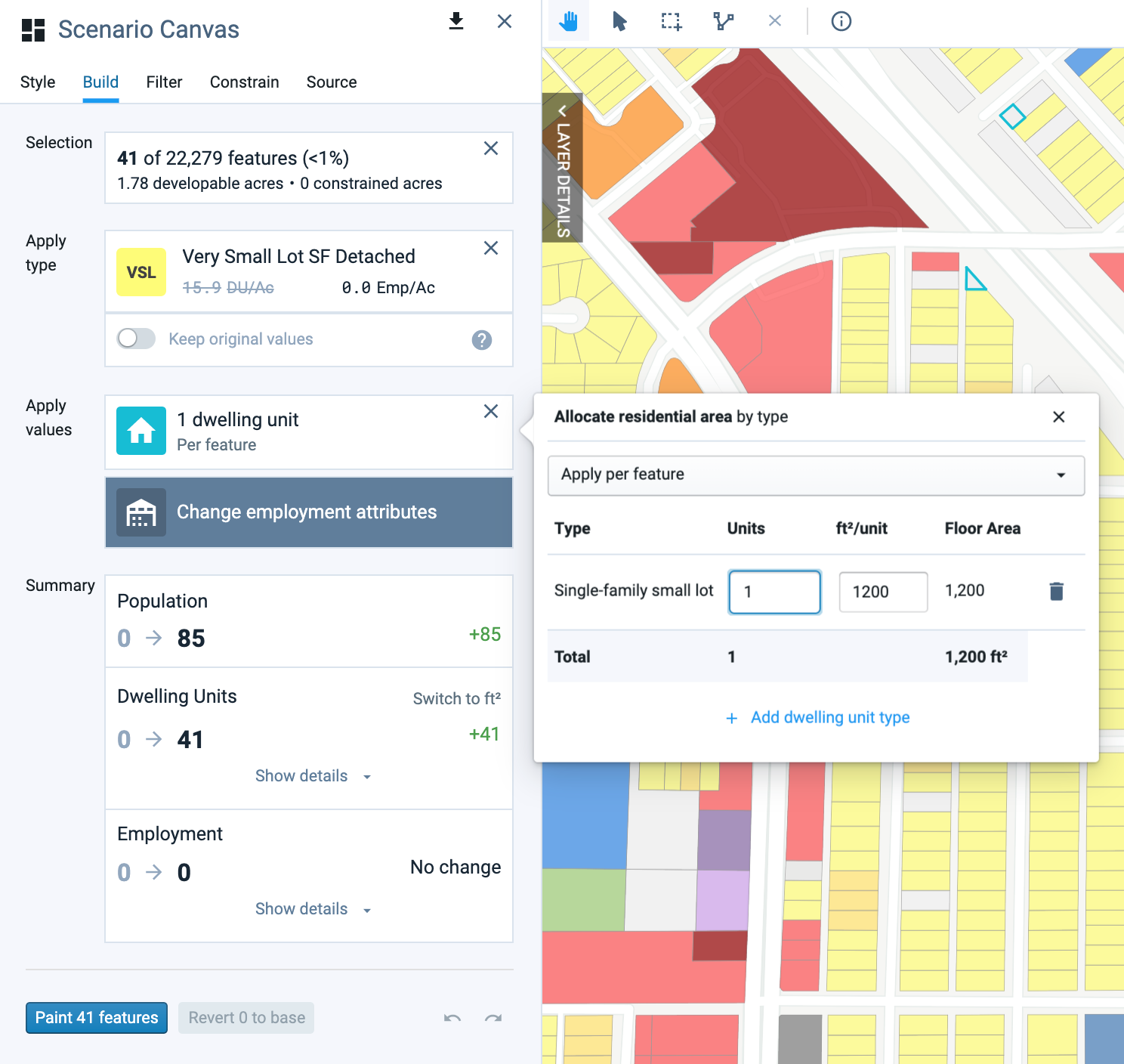
Entering residential attributes
The Summary section will be updated to show the 41 dwelling units and associated population. The population is calculated using the project-wide variables for the average single-family small lot household size and overall residential occupancy. These variables are set on the Library Settings page in Manage mode.
Click the X button at the top right of the Allocate residential area by type window to close it. Your entries are automatically saved.
Click the Paint x features button. The features will be painted, with changes reflected in the scenario canvas summary charts, on the map, and in the data table for the scenario.
Manage and Monitor Painting Actions
If needed, you can undo or redo your painting actions, or revert features to their base condition. The Scenario Canvas Summary Charts in Build mode, Summary Statistics in Report mode, and the data table all provide scenario-wide information to track the growth you have painted.
To make any changes, use the Revert x to base, Undo
, or Redo controls. Reverting effectively returns features to their base condition. Undo and redo are applied to your sequence of past actions, independent of the features that are currently selected.As you continue to select and paint features, track scenario development progress using the scenario canvas summary charts. This is useful if you are building scenarios to meet control totals for new growth.
Enter Report mode and select Summary Statistics to view comparative statistics for your scenario. The charts in this mode allow you to compare scenarios with each other.
Enter Analysis mode and run analysis modules as needed. You can run analysis to gauge impacts, for example land consumption, as you develop a scenario. Note that once you make land use changes any prior analysis runs will become outdated; the status as to whether results are current or outdated is indicated in Analysis and Report modes.
Depict Master Plans
Analyst can be used to depict development according to master plans or other project-level proposals for large existing sites. By "gridding" parcel features in the Base Canvas, you can paint future development characteristics at a finer resolution than that of existing features.
In this tutorial, we'll use the Base Canvas feature gridding controls to split a large redevelopment site into a grid of smaller parcels, then paint development onto the new parcels. As part of this process, it's helpful to be familiar with land use types and the scenario painting process. See the previous tutorials on creating Components and types, and painting scenarios, for guidance.
Data Layers | Features |
|
Feature Gridding
Open or create a new project containing a large development site to work with. For our example, we'll look to the proposed Sunnyside Yard Master Plan—a plan for 140 acres of development above a passenger rail yard in Sunnyside, Queens.
Note
Feature gridding is applicable for projects created on or after May 1, 2020. Unfortunately, it cannot be applied in older projects. To enable feature gridding, we recommend that you create a new project.
Open the Edit tab for the Base Canvas. The Edit tab of the Layer Details pane contains the feature gridding controls. From here, you can also remove features.
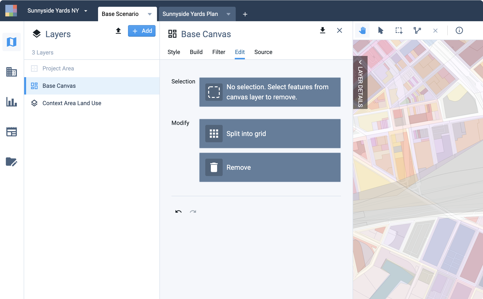
Feature gridding controls located on the Base Canvas Edit tab
Select canvas feature(s) to be split into grid cells. Use the manual selection tools to select one or more parcel or block features. You can work a single feature, or multiple features at once. For our example, we'll split up the two existing parcels comprising the Sunnyside Yard area.
Selecting two parcels on the Base Canvas to be split
Click Split into grid. The Split into grid window will appear.
Previewing the grid layout
Configure the grid layout. The grid configuration settings allow you to control the size, angle, and horizontal and vertical offsets of the grid layout.
Enter a grid cell size. You can specify a size in terms of area or grid cell edge length. Use the dropdown list to select a unit of measure, then enter a value. You'll see a preview of grid lines drawn onto the selected feature, and the resulting count of new features will be shown at the bottom of the window.
For our example, we'll set the grid cell edge length to 300 feet to align with the standard block size and right-of-way width indicated in the master plan.
Setting a grid cell size
In our example, we're setting up the grid cells to represent gross area inclusive of rights-of-way. In other words, right-of-way area is distributed among the new features. In this case, we'll need to paint them using Place Types that incorporate assumptions for right-of-way area.
As an alternative, you could set up grid cells to represent net area, and paint buildings and rights-of-way separately using Building Types. Painting grid cells as rights-of-way is another way of representing the amount of land dedicated to streets and sidewalks. (Note that the particular location of features designated as right-of-way areas will not affect transportation and accessibility analysis since they will not be recognized as functional street networks.)
You can grid features into a maximum of 500 new features; a warning will appear if your grid cell size would result in too many. To create more features of a smaller size, try gridding one feature at a time. If you're already working with a single feature, you can perform successive gridding operations: first, split your parcel or block into two or more large features by using a large grid cell size; then, split the resulting features into smaller grid cells.
Adjust the angle of the grid. Use the slider control or enter a value in degrees—negative values rotate the grid to the left, positive values to the right. Use the preview to set the grid angle as desired. For our example, we'll set the angle to align with the illustrative of the master plan.

Adjusting the angle of the grid layout
Adjust the horizontal and vertical offsets. The offsets shift the entire grid layout horizontally and vertically. Use the slider controls, or enter values in terms of the percentage of the grid cell edge length.

Using the horizontal and vertical offsets
Click Apply to grid the feature into cells as shown. The original feature will be split out into new features. The new features will register on the map and show up in the data table.
Applying the grid layout
Each new feature will retain the land use classifications of the original feature, with population, households, dwelling units, jobs, and building attribute values distributed among the new features in proportion to their land area.
When complete, the effects of splitting features will be reflected in summary charts for the Base Canvas and any scenarios. If you split a feature that had previously been painted in a scenario, the feature will be replaced with the new gridded features as depicted in the base, with paints maintained.
Gridding features also renders any prior analysis runs as out of date, so you will need to re-run analysis afterwards. The status as to whether results are current or outdated is indicated for each module in Analyze and Report modes.
Continue gridding features as needed. Newly gridded features can themselves be gridded into smaller features. You'll see a depiction of nested splits in the painted example that follows.
Use the Undo
or Redo controls to make sequential changes, if needed. Undo and redo apply to your sequence of past feature gridding, feature removal, and painting actions, independent of the features that are currently selected.You may choose to undo a gridding operation so you can change the grid layout, or otherwise restore the original feature geometry. If you do so after having painted any new gridded features, be sure to check how the features are affected in your scenarios. Paints applied to any gridded features may be extended to the entirety of the original feature if a gridding operation is reversed. If this is not intended, you can re-paint features or revert them to their base condition.
Edit the new gridded features in the Base Canvas, if needed. The gridding operation distributes existing population, households, jobs, and development among the new gridded features to maintain the totals from the original feature. You can use the Base Canvas editing controls to make any desired adjustments to the land use designations and/or development characteristics of the new features as depicted in the Base Canvas.
Paint a Master Plan
Once you have edited your Base Canvas to include new gridded features, you can paint them to represent site plans.
Create a new scenario, or work within an existing scenario. If you created a scenario prior to gridding features, the scenario canvas will be updated automatically to include the new features.
Enter Build mode for the scenario.
Paint the new features to represent plans. You can paint newly gridded features like any other in the canvas. For our example, we've painted the newly gridded features with Place Types to broadly represent the Sunnyside Yard Master Plan. The features represent gross land area for city blocks (with an average size just over two acres), large open space areas, and the rail yard. You can see the illustrative plan and the scenario depiction below.
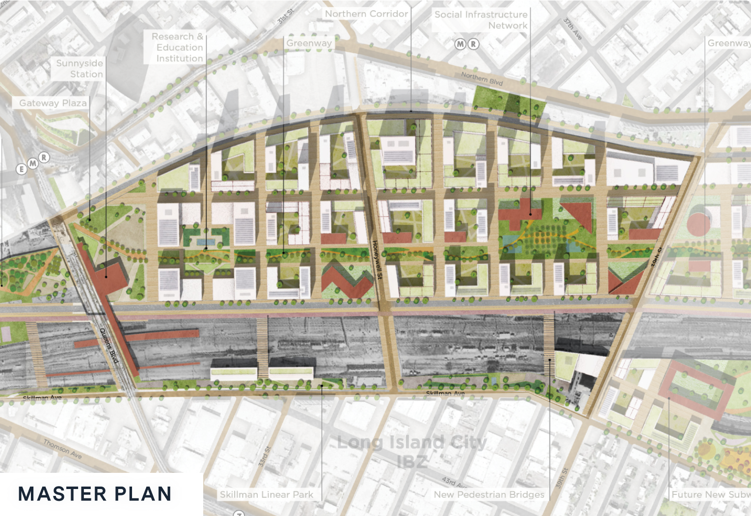 |
Illustrative from Sunnyside Yard Master Plan
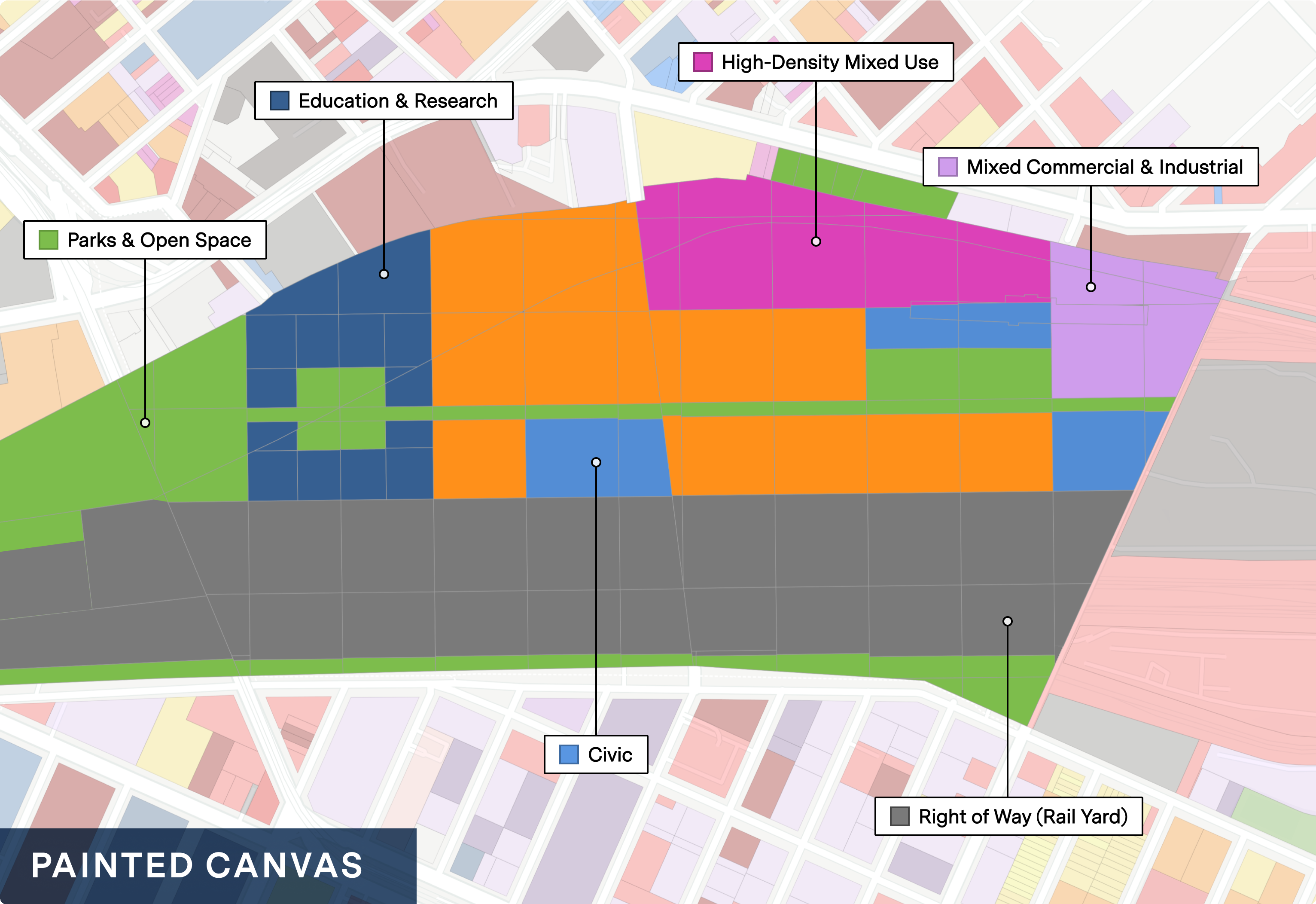 |
Gridded features as painted in a scenario
In the example, the features representing individual blocks are painted with Place Types reflecting different areas of the plan, including a high-density mixed use area, a commercial cluster, an educational institution, civic commons and open spaces, and a "neighborhood fabric" area. We used Place Types to incorporate a range of Building Types—for example, a mix of low-, mid-, and high-rise buildings—and civic components such as schools and parks throughout the plan area. Rights-of-way are also built into the Place Types, while the rail yard area is painted directly as a right-of-way type. The Place Types can be defined with a mix of Components and Building Types to reflect the proposed development program, which indicates ranges for new homes, jobs, and building and land area by use.
Going beyond this example, there are many options for how you might use feature gridding and scenario painting to represent plans. For smaller-scale plans in which gridded features are set up to represent individual parcels, painting with Building Types would be appropriate. Feature gridding can also be applied to represent development in the context of large block-based projects—for example, to depict greenfield growth over land areas smaller than a full census block. For more help in understanding how feature gridding can support your work, please contact Analyst support.
Set Analysis Module Parameters
Analysis module parameters are variable input assumptions used to localize analysis and test technology or policy-based targets into the future. Parameters can be varied by scenario, allowing you to test different configurations of assumptions in concert with land use alternatives. Each module comes loaded with a set of default assumptions, which can be changed based on your own data sources.
In this tutorial, we'll walk through the basic steps of setting analysis parameters. See the Features documentation for a summary of the analysis parameters, and links to the analysis module methodologies for more detailed information about the module parameters and how they are applied.
Data Layers | Features |
None |
Enter Manage mode by clicking the Manager mode button
in the Mode bar. The Manage mode screen appears.Click the Analysis Modules tab, if it is not active already. The Analysis Module Parameters screen appears.
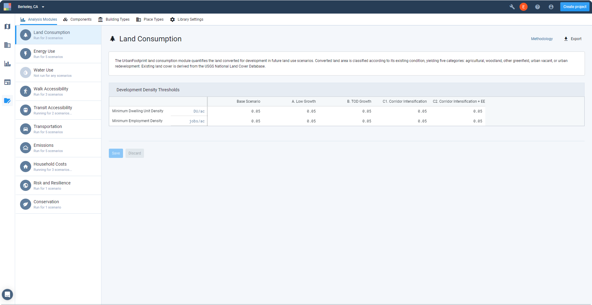
Analysis Module Parameters screen
Select a module from the list at left. The parameter screen for the module appears.
Double-click on values to edit them. Manually enter or adjust values as needed. Edited values appear in blue text.
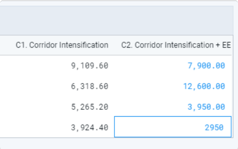
Edited parameter values
Click Save to save your edits. Otherwise, click Discard to revert values to their previous state.
Run (or re-run) the analysis module to see results. Changing the analysis parameters of a scenario renders any previous analysis as out of date. The module must be run again to apply the new parameters.
To save a copy of the analysis assumptions, click the
 Export button in the upper right corner of the screen. An Excel spreadsheet containing the current module's analysis parameters for all scenarios is downloaded to your computer.
Reset Parameter Values back to their Defaults
Roll over the header for a group of values in a scenario and click the expand menu button
 that appears.
Select Reset to defaults. The selected group of parameter values are reset to the defaults.
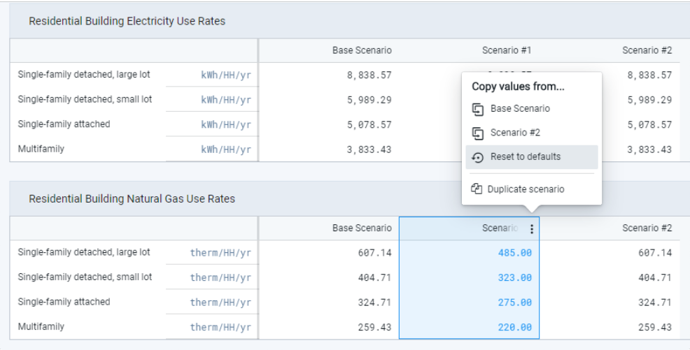
Resetting parameters to use default values
Click Save to save your edits. Otherwise, click Discard to revert values back to their previous state.
Copy Parameter Values between Scenarios
Hover over the header for a group of values in a scenario and click the expand menu button
that appears.Select the scenario from which you want to copy values. The group of parameter values from the selected scenario are copied over.
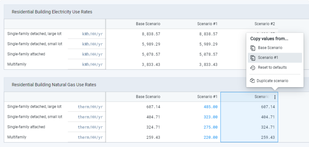
Copying parameter values from one scenario to another
Click Save to save your edits. Otherwise, click Discard to revert values to their previous state.
Analyze a Scenario
Analyst produces comprehensive analysis of scenarios based on variations in land use and development in combination with analysis assumptions that can be linked to policy or technological change. You can run analysis on the base or future scenarios at any time to produce mapped output layers, in-tool reports, and data exports.
In this tutorial, we'll enter Analyze mode to run analysis modules. For information on varying analysis parameters for scenarios, see Set Analysis Parameters.
Data Layers | Features |
Scenario upon which to run analysis |
Select a scenario to analyze. Click the tab of the scenario for which you would like to perform analysis. Modules are run for individual scenarios.
Enter Analyze mode. Click the Analyze mode button
 in the Mode bar. The Analysis Modules pane appears. All available modules are listed, and the current state of each is indicated.
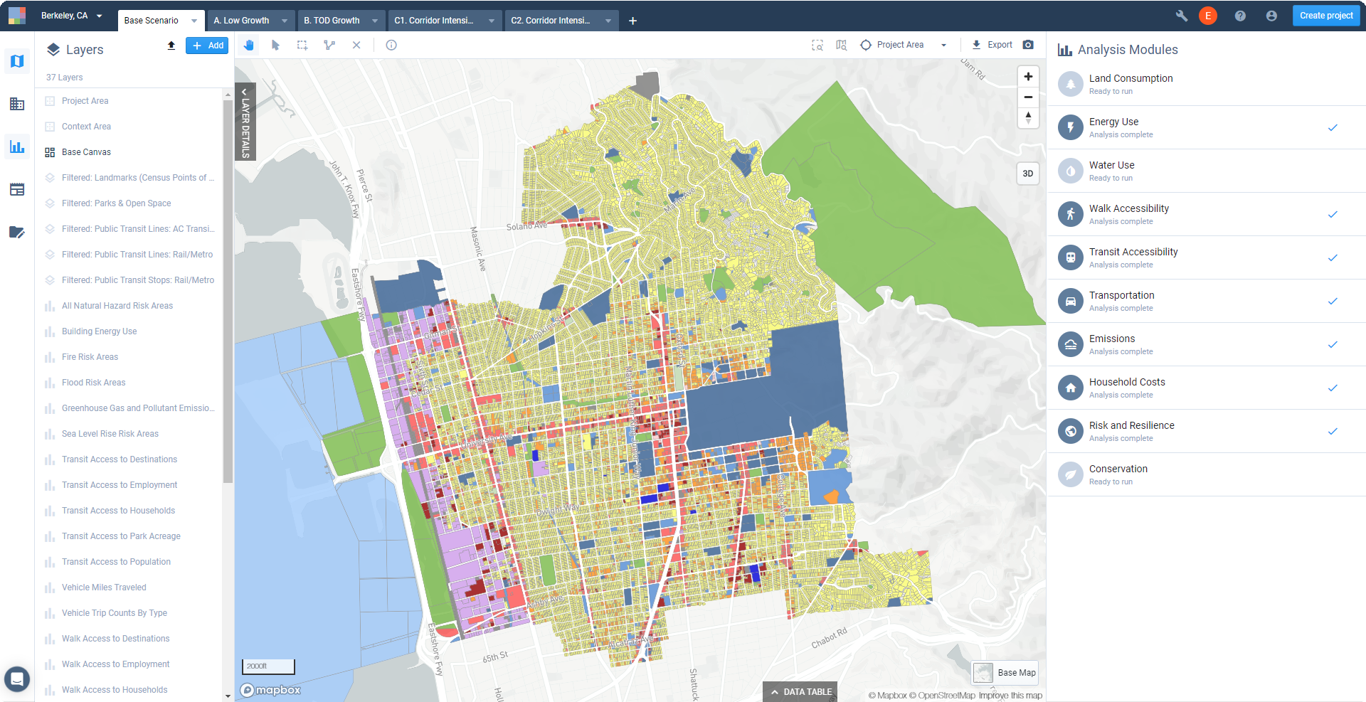
A view of Analyze mode
Ready to run indicates that analysis has not yet been run.
Analysis complete indicates that a module has been run and the results are up to date.
Analysis out of date alerts you that a module has been run, but changes have since been made to the scenario's land use or analysis parameters; in this case, analysis needs to be re-run to update the results. Updating the Base Canvas will render all modules in all scenarios out of date.
Run analysis for individual modules. Hover over the analysis module you want to run and click the Run analysis button
 . The module will start running. As it runs, you will see an in-progress indicator. When complete, a checkmark will appear. You can then view your results.
Note
Analysis run times vary according to the size of your project and the complexity of the modules, with some requiring a few minutes or more. While you wait, you can continue using other features in the platform, switch to another project, or even close Analyst.
Analysis results can be viewed on the map and data table, via charts for the current scenario, or via charts in Report mode that compare results across multiple scenarios. See Work with Analysis Module Outputs for details on viewing results.
Run other analysis modules as needed. Modules can be run simultaneously. Switch scenario tabs and follow the same process to run analysis for other scenarios.
Measure Walk and Transit Access to Custom Points of Interest
The Walk and Transit Accessibility modules measure access from each canvas feature to households, employment, and destinations including schools, parks, hospitals, retail locations, and transit stops. With the ability to set custom points of interest (POIs), you can expand your accessibility analysis to include new destinations. Any layer consisting of point features can be used as an input.
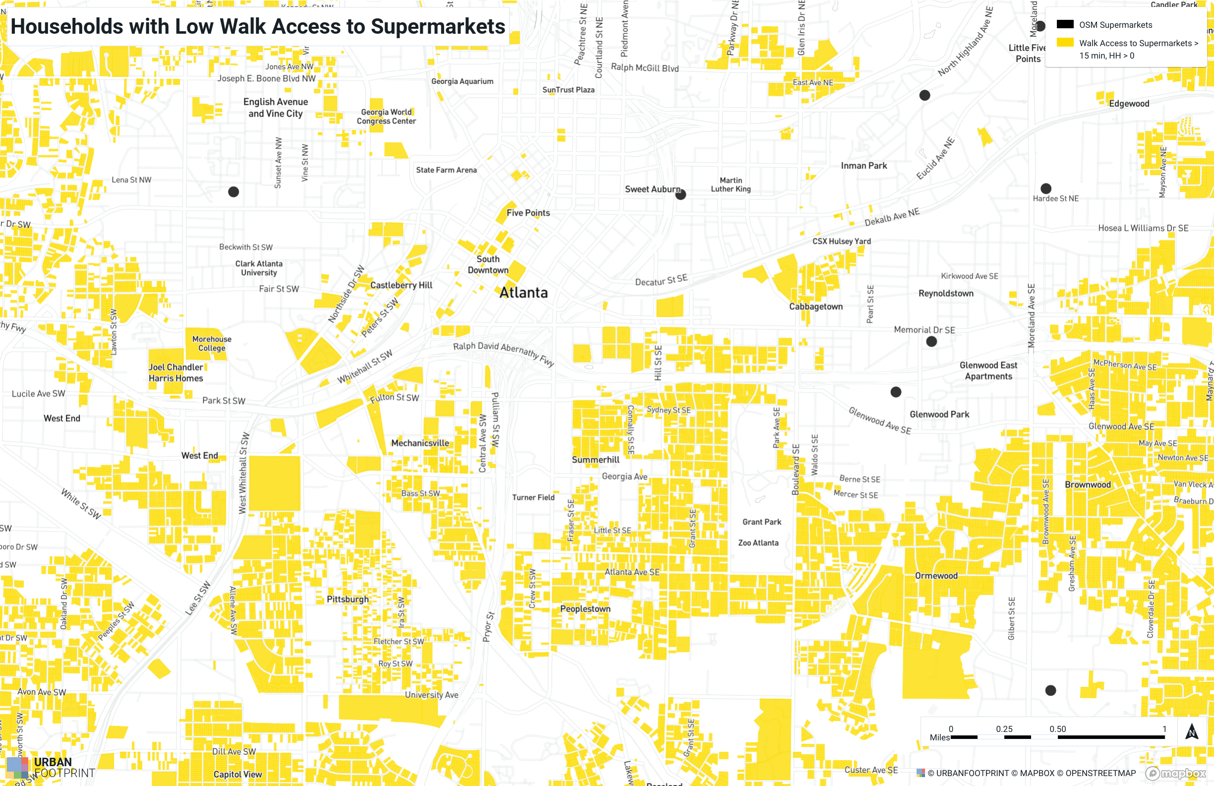 |
Households in areas with over 15-minute walk access to supermarkets in Atlanta neighborhoods
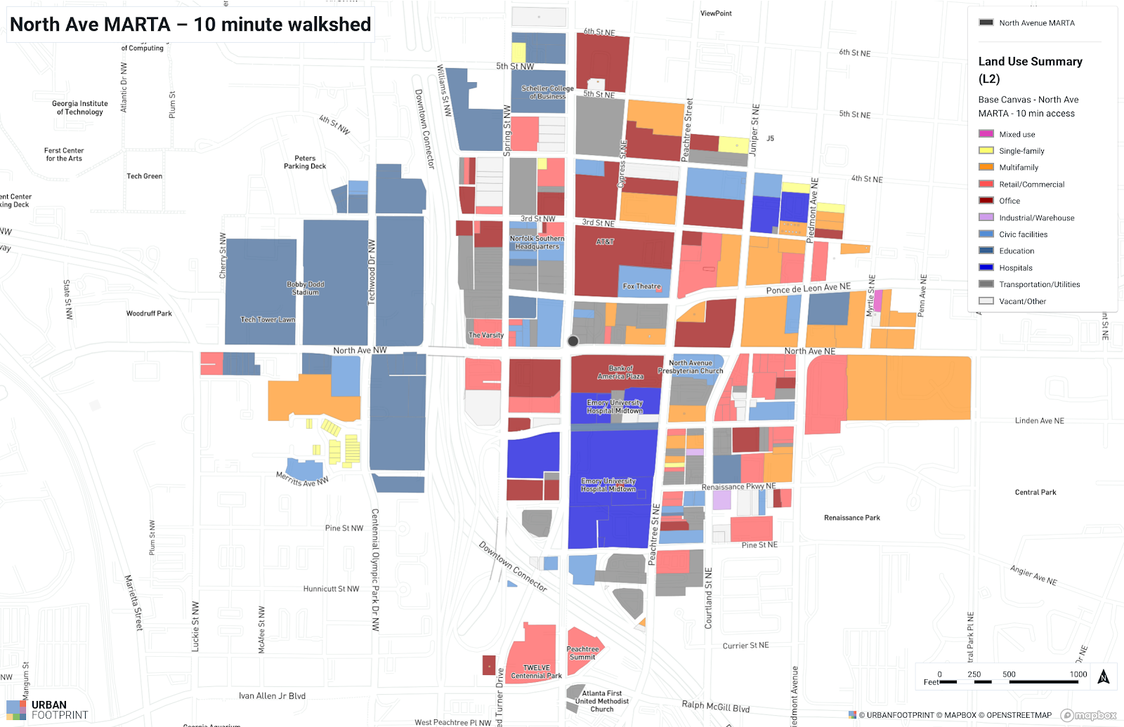 |
Base Canvas land use in the 10-minute walkshed of the North Avenue MARTA station in Atlanta
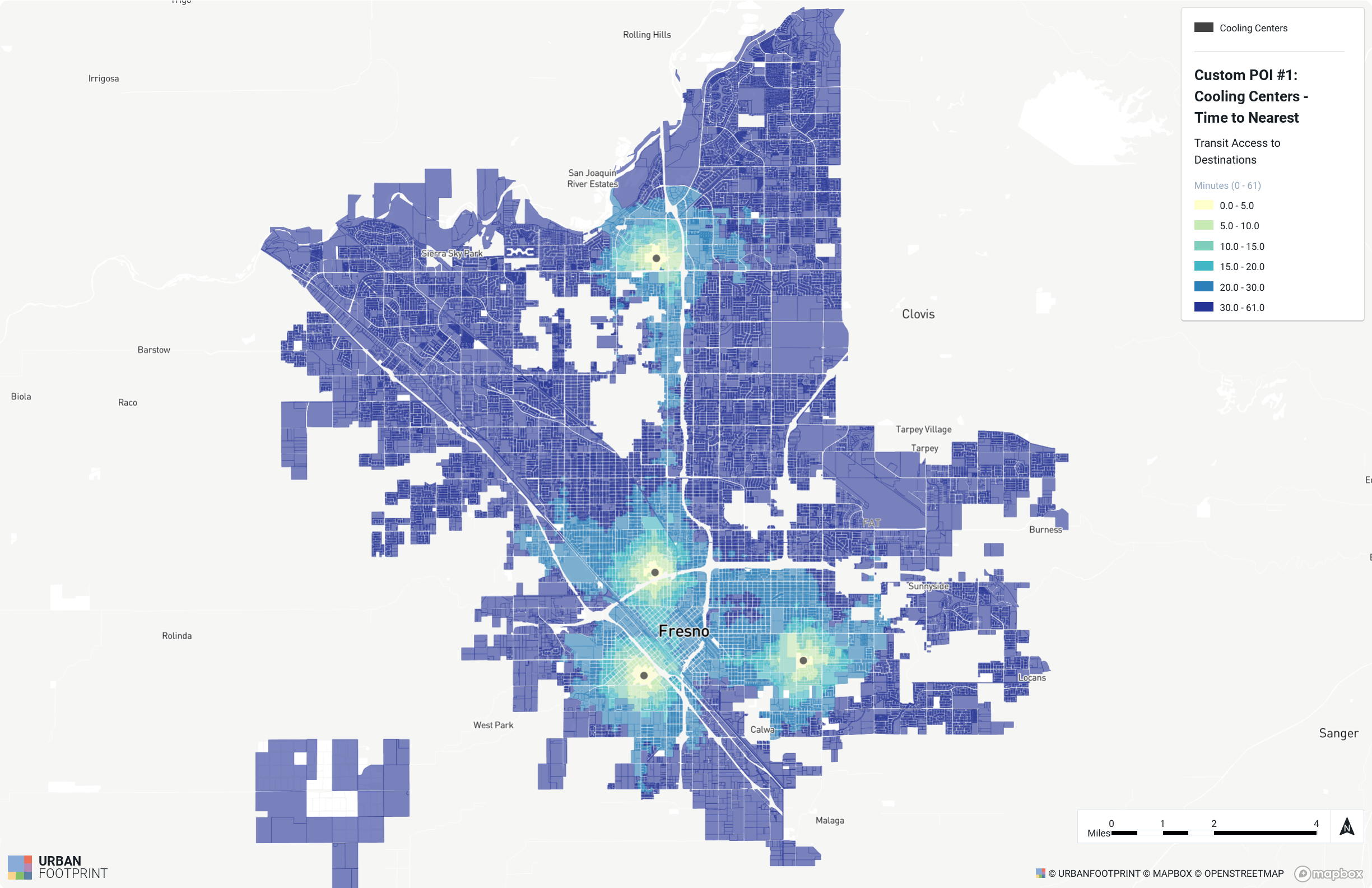 |
Transit access to cooling centers in Fresno
Data Layers | Point layers representing destinations |
Features |
Measure Access to Supermarkets
This example steps through the basics of running an accessibility analysis to custom points of interest, then filtering the output and joining with other layers to identify where low accessibility coincides with other criteria.
Add or upload a layer containing the custom points of interest. Custom POI layers must consist of point features (not lines or polygons). For our example, we'll use the OSM Supermarkets reference layer. Add it to your project using the Layer Manager; see Use Reference Data for details on adding layers.
If you have a point layer from outside Analyst to use, upload it by clicking the Upload Layer button
 in the upper right portion of the Layers pane. See Upload Data Layers for details on uploading layers.
The accessibility modules will measure access to all points in the selected layer. If you wish to measure access to only a selection—for example, those of a specific type or value range—select features using filters and/or the manual selection tools as needed and save as a new filtered layer (see Filter and Join Data for details). Then, you can choose the saved filtered layer as the custom POI input.
Note
While you cannot create new point features in Analyst, you can quickly generate point data layers in GeoJSON format at geojson.io. See Create Custom Layers in GeoJSON Format for details. You can also use a standalone GIS tool to create point datasets.
Navigate to the Walk Accessibility module inputs in Manage mode.
Enter Manage mode by clicking the Manage mode button
in the Mode bar.Click the Analysis Modules tab, if it is not active already.
Select the Walk Accessibility module from the list on the left. For our example, we'll set custom POIs for the Walk Accessibility module. The parameter inputs for the Transit Accessibility module follow the same format.
Enter parameters for your custom POIs. Find the input parameters in the Custom Point of Interest Attributes parameter section. You can select up to three custom POIs for each scenario. The POIs do not need to match across scenarios. (If you need to measure access to more than three POIs for the base or a scenario, you can duplicate it and specify additional POIs to apply in the duplicated scenario.)
Note that you can also adjust the average walk speed.
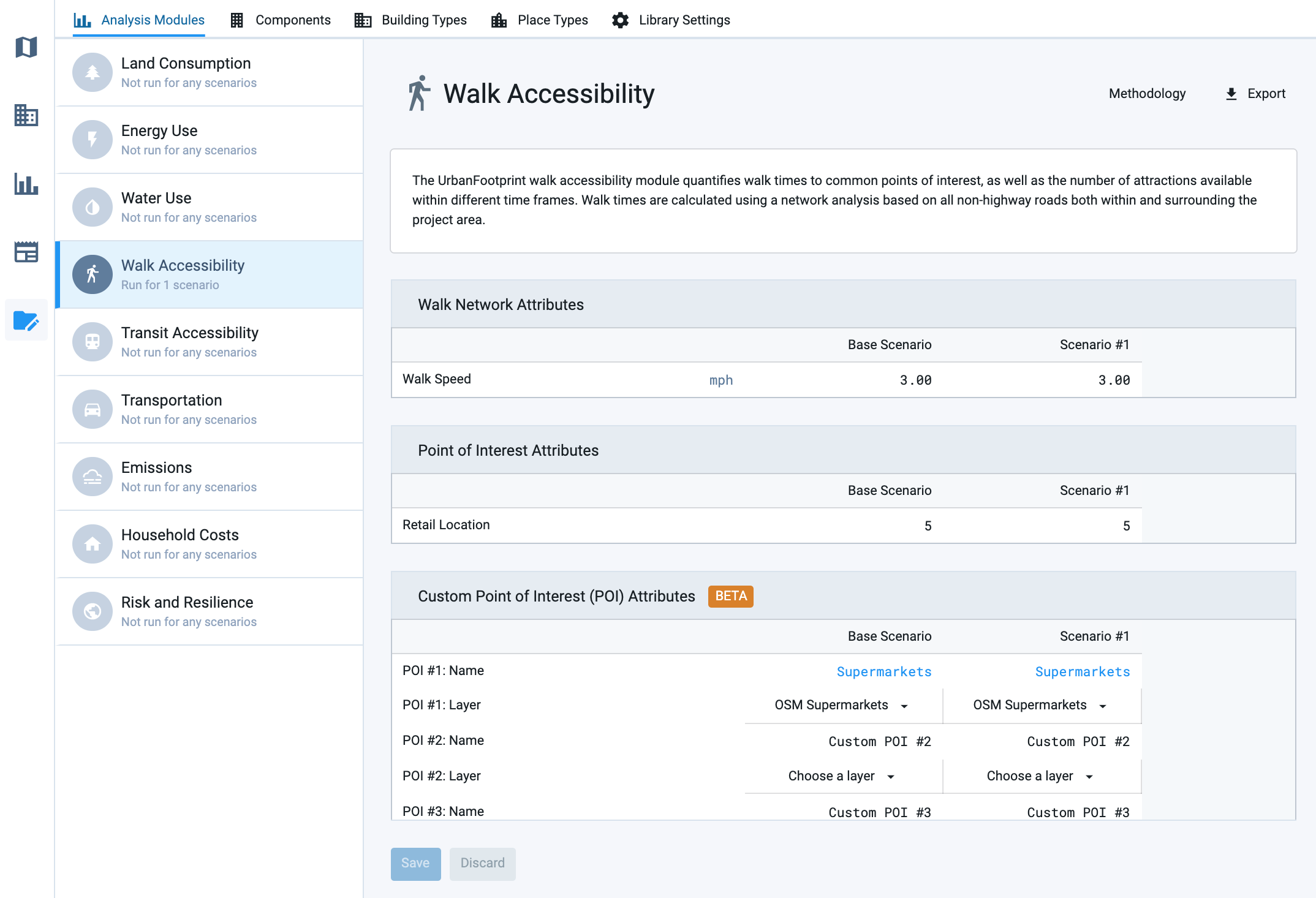
Setting custom points of interest in Manage mode
For each custom POI that you would like to include, enter a name. POI names appear in the headers of the results charts, and in the column names of the analysis output layer. Double-click on the default name (e.g., Custom POI #1) to edit it. Edited values appear in blue text.
For each custom POI, select a layer. The drop-down list allows you to select from the point layers loaded to your project. Find the layer(s) that you added, uploaded, or saved. If an intended layer does not appear in the list, verify that it contains point features, rather than polygons or lines.
Click Save to save your edits. Otherwise, click Discard to revert the inputs to their previous state.
Run the Walk Accessibility module. From Analyze mode, run the Walk Accessibility module for the scenario(s) for which you specified the supermarkets and any other custom POIs. Changing the analysis parameters of a scenario renders any previous analysis as out of date, so if you ran the module previously you'll need to run it again to apply the new parameters.
Explore the accessibility results. The results for custom POIs can be found alongside the other destination access results in the summary charts and the Walk Access to Destinations map layer and data table.
View the results chart in the Analysis pane, which indicates the percentage of residents in the project area within a 5, 10, 15, or 20 minute walk to a supermarket.
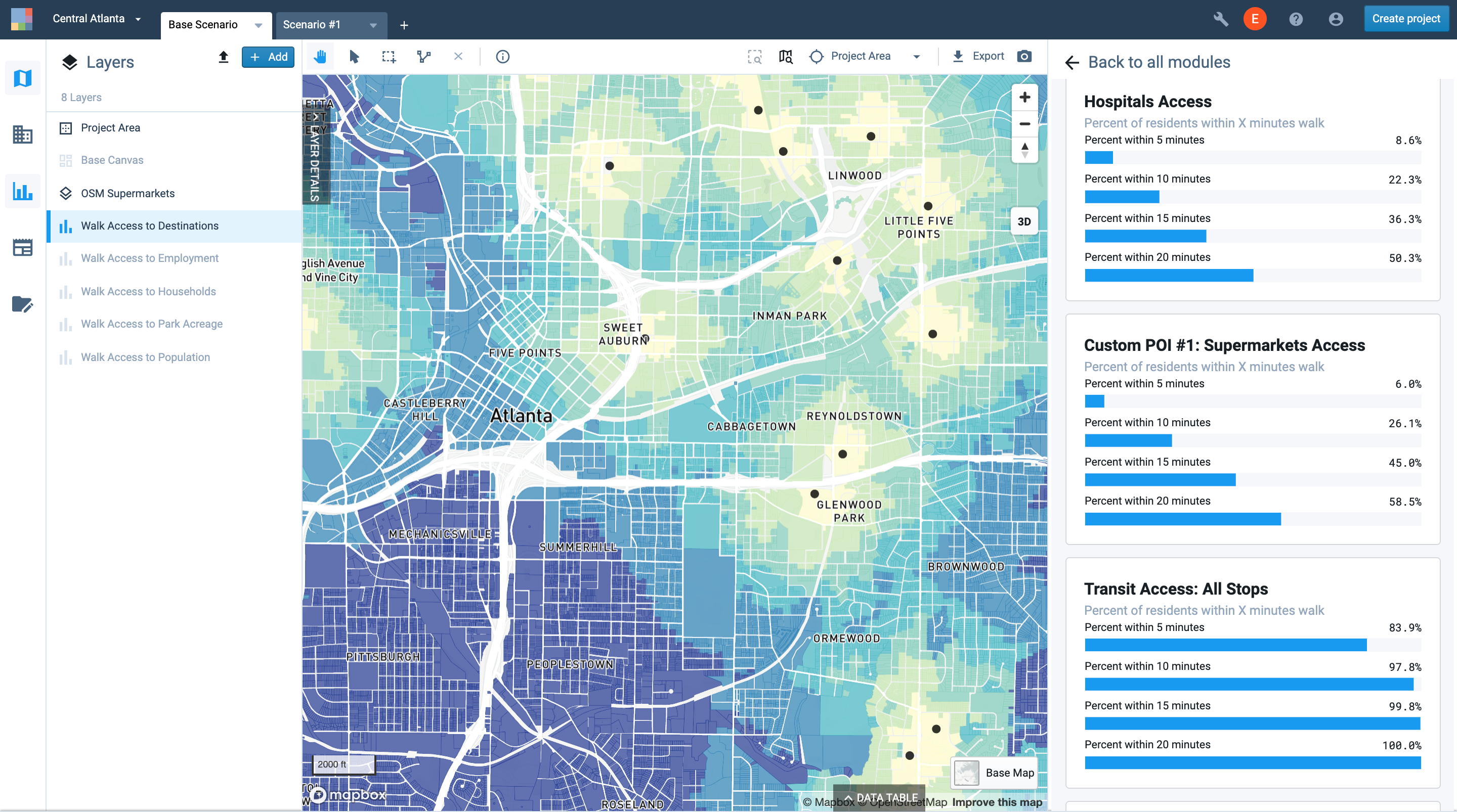
Viewing Walk Accessibility results charts in Analyze mode
View the data table for the Walk Access to Destinations layer, which contains a column for each custom POI. Results are expressed in minutes to the nearest destination.
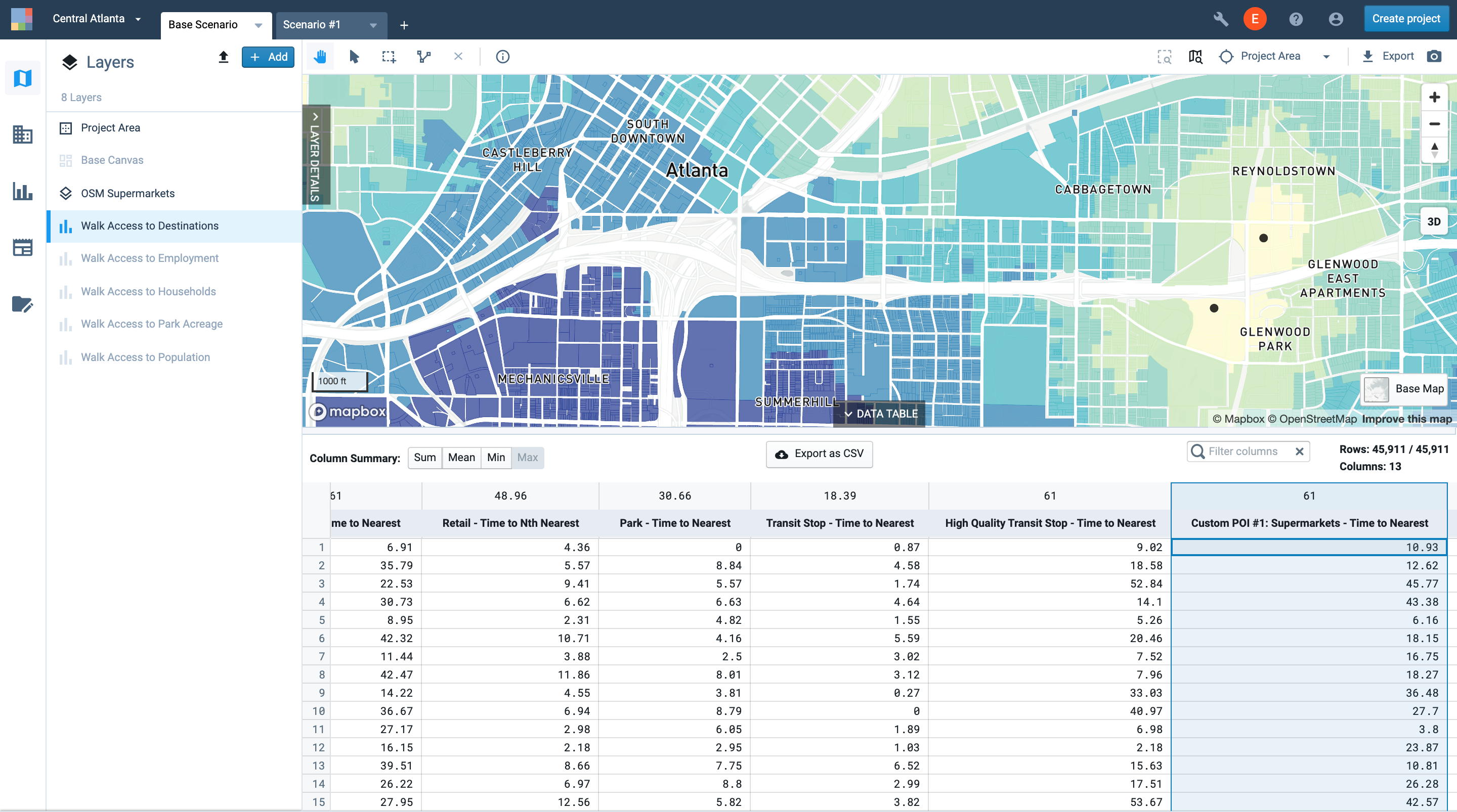
Map the accessibility results by selecting the custom POI column in the Walk Access to Destinations layer.
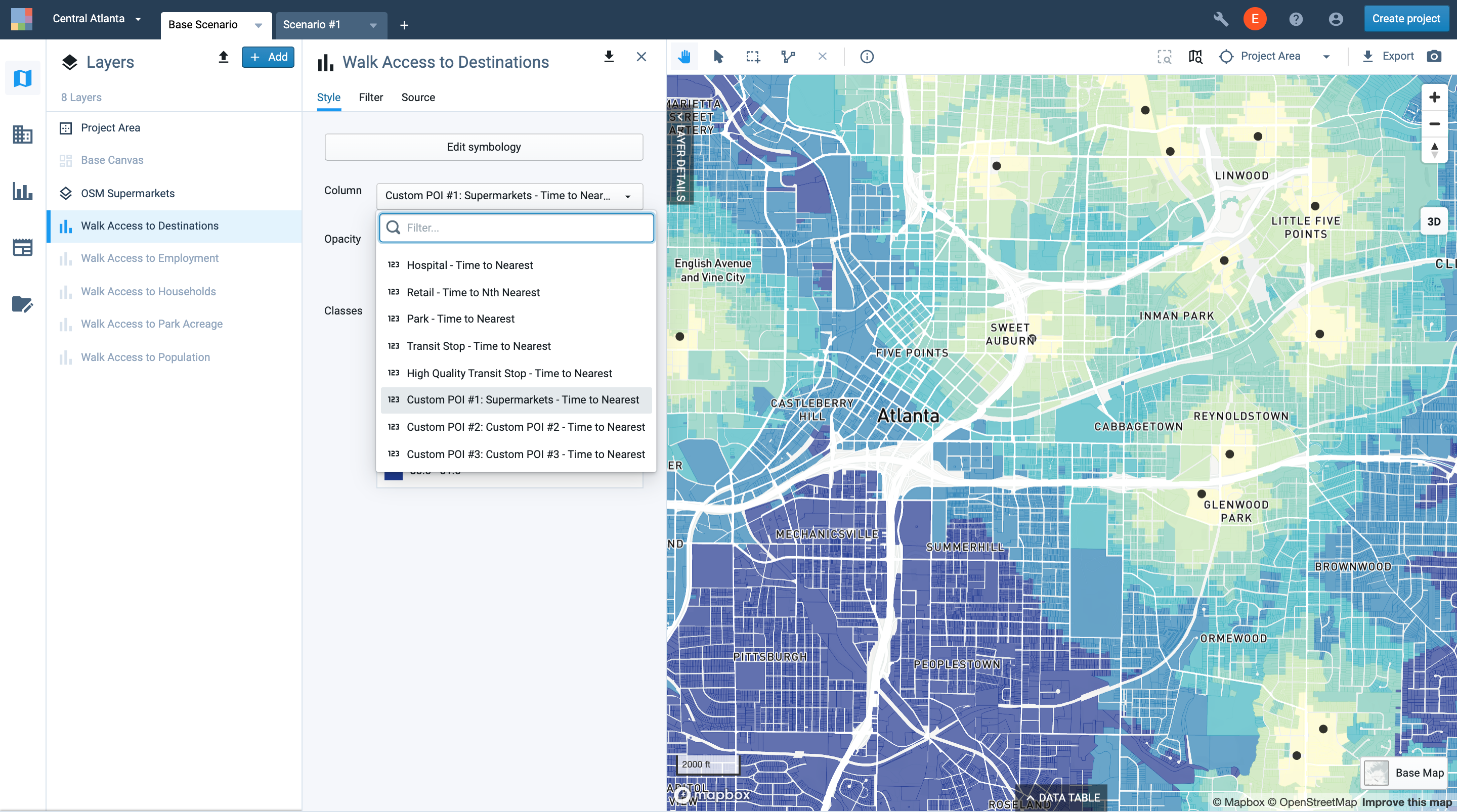
Select the custom POI column for display
You can edit the layer symbology to adjust the classes and colors displayed.
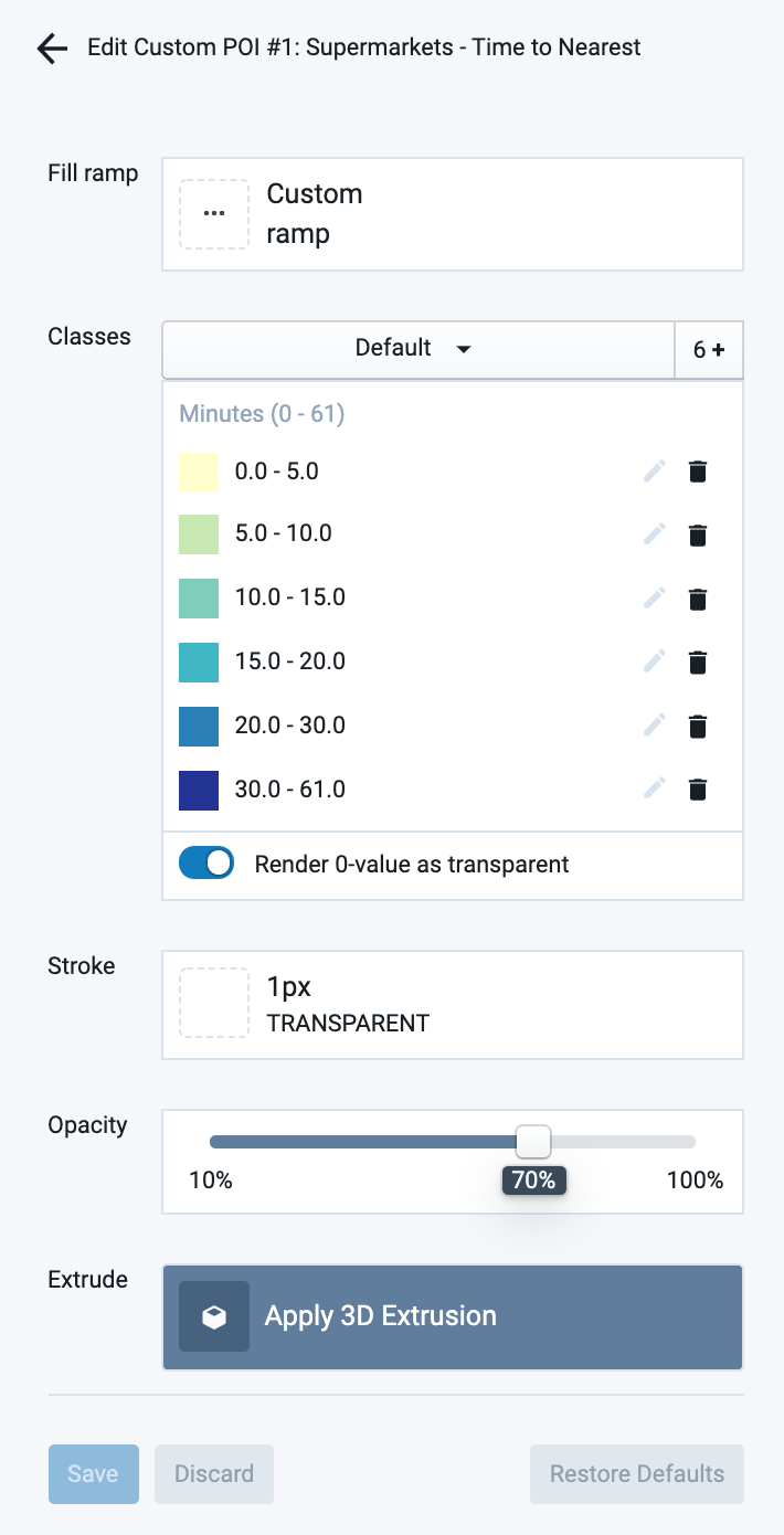
Default classification for access to custom POI destinations
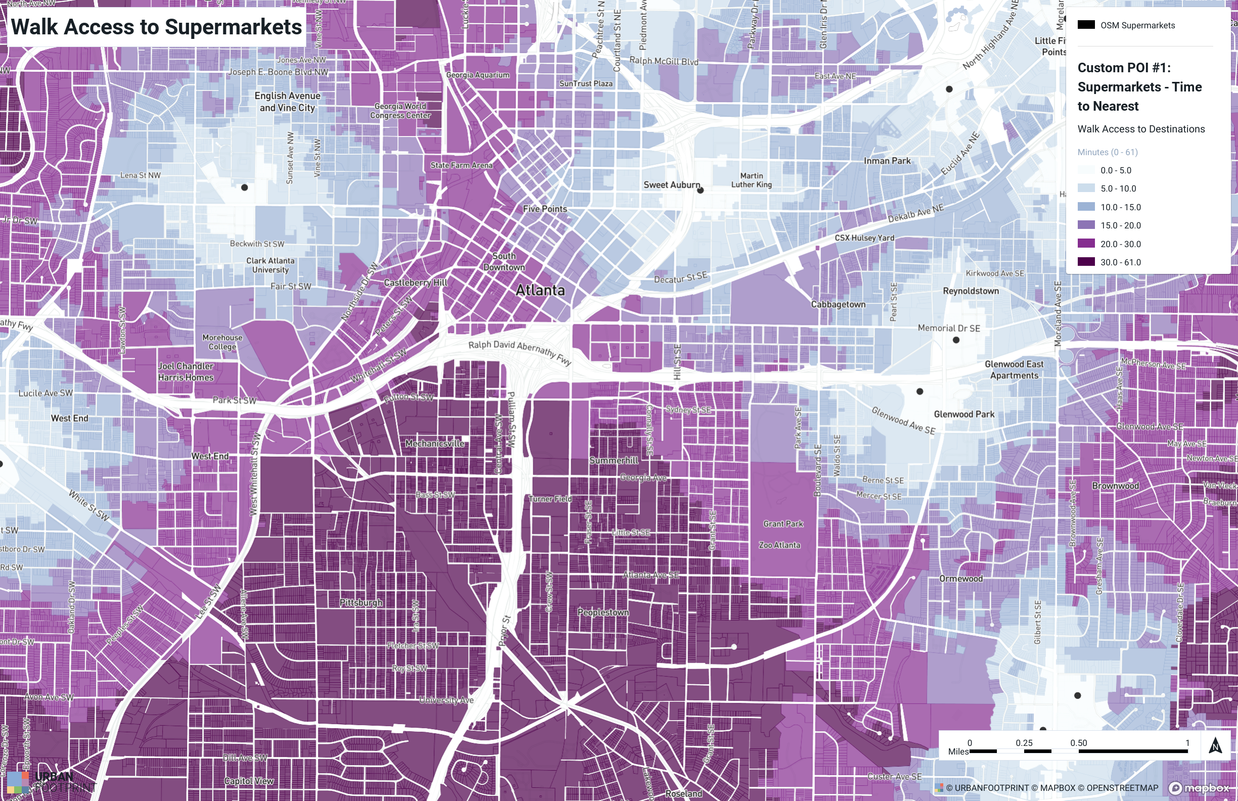
Map of walk access to supermarkets in Atlanta
Summarize population, households, or employment within access areas. The Walk Access to Destinations layer contains population, households, and employment counts for each canvas feature. You can apply filters and joins to quantify, for example, the percentage of households within a neighborhood that lacks walkable access to supermarkets.
Click the Filter tab for the Walk Access to Destinations layer.
Click Add filter +, then select the custom POI output column (in this case, "Custom POI #1: Supermarkets - Time to Nearest") and specify an access range, in minutes. We'll select all parcels within a 0 to 15 minute walk of a supermarket.
Click Join layer, then select a join layer and add filters to it as needed. For our example, we'll use a saved filtered selection of the Neighborhood Boundaries reference layer and select a single neighborhood. See the filter and join selections below.
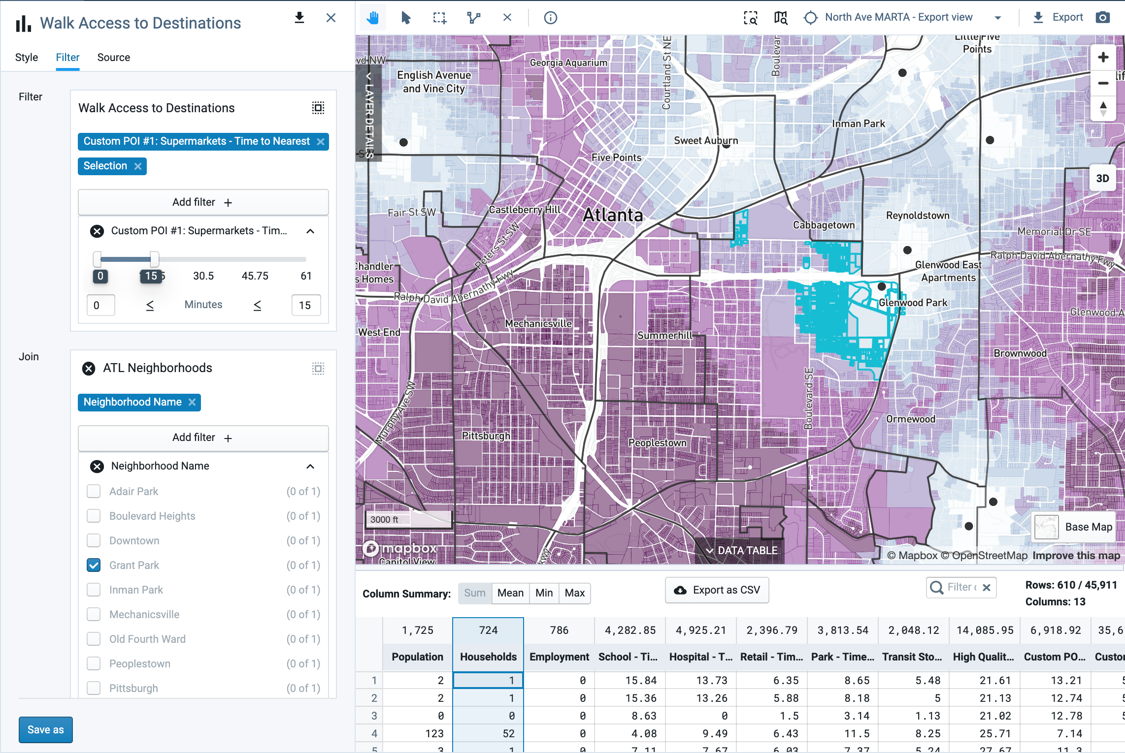
Using filters and joins to select parcels within a 15-minute walk of a supermarket in a neighborhood
View the data table for a summarized result. The column summary for the Households column can show the sum total within the selected parcels. For our example, we can see that there are 724 households within a 15-minute walk of a supermarket in the Grant Park neighborhood.
Remove the filter for the POI access criteria to select all parcels in the neighborhood. According to the data table, this yields a total of 2,908 households.
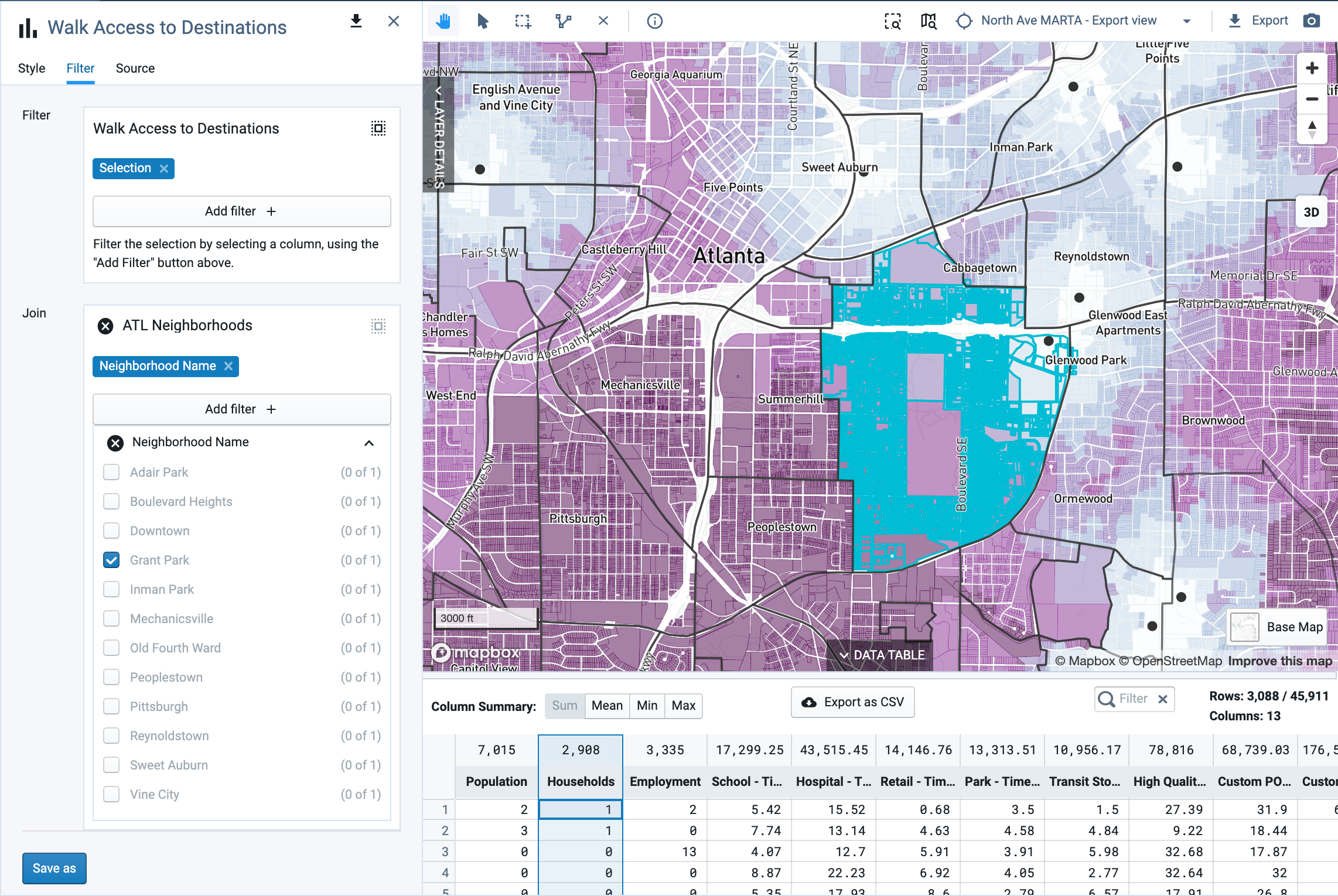
Selecting all parcels within a neighborhood
We can now calculate that 25% of households in the Grant Park neighborhood have 15-minute walk access to a supermarket, while 75% do not. Based on the map view, we can also see that the nearby neighborhoods of Pittsburgh, Mechanicsville, Summerhill, and Peoplestown have much lower access, with no supermarkets within a reasonable walking time.
Use the custom POI accessibility outputs in further analysis. You can perform further analysis using filters and joins with other layers to identify where households have low access and fulfill other criteria. For example, the map below was generated by using the HUD Low Poverty Index reference data layer to select households with low supermarket access in areas with low index scores, indicating high poverty. We can see that walk access to supermarkets is most deficient in high-poverty neighborhoods.
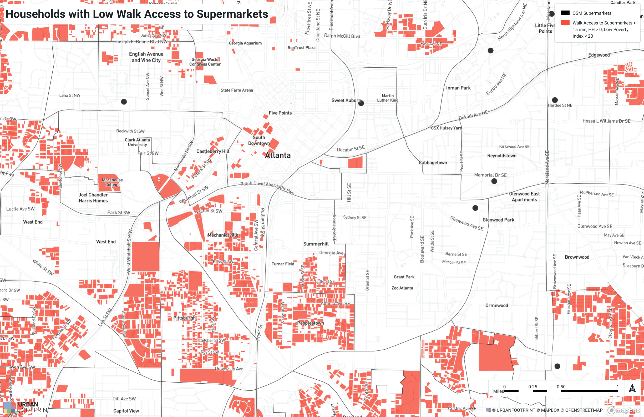
Households in areas with high poverty and low walk access to supermarkets
Perform Walkshed Analysis
Custom POI accessibility analysis can also be used to generate walksheds around individual points such as transit stations or development sites. Using walksheds, you can identify places in other layers to and from which you can reach a selected point—for example, bike stations that fall within a 5-minute walk of a particular transit station. You can also quantify attributes of those places, such as office employees within the walkshed according to the Base Canvas or scenarios.
In this example, we'll run custom POI analysis to delineate a walkshed around an existing transit station, which we'll then join to the Base Canvas for mapping and analysis.
Create a saved selection for the custom point of interest. We'll focus on the North Avenue MARTA station in Atlanta. From the Public Transit Stops reference layer, select the station using the point selection tool
 , then save the selection as a filtered layer. (See Filter and Join Data for details on saving filtered layers.) We'll call the layer "North Avenue MARTA."
Navigate to the Walk Accessibility module inputs in Manage mode.
Enter Manage mode by clicking the Manage mode button
in the Mode bar.Click the Analysis Modules tab, if it is not active already.
Select the Walk Accessibility module from the list on the left.
Enter parameters for the custom POIs. Find the input parameters in the Custom Point of Interest Attributes parameter section. You can select up to three custom POIs for each scenario, so if you were working with multiple individual transit stations you could select them as other POIs.
Enter a name for the transit station POI. Double-click on the default name (e.g., "Custom POI #1") to edit it. We'll enter "North Avenue MARTA."
Select the transit station layer as the custom POI. The drop-down list allows you to select from the point layers in your project. Find your saved layer—in this case, "North Avenue MARTA."
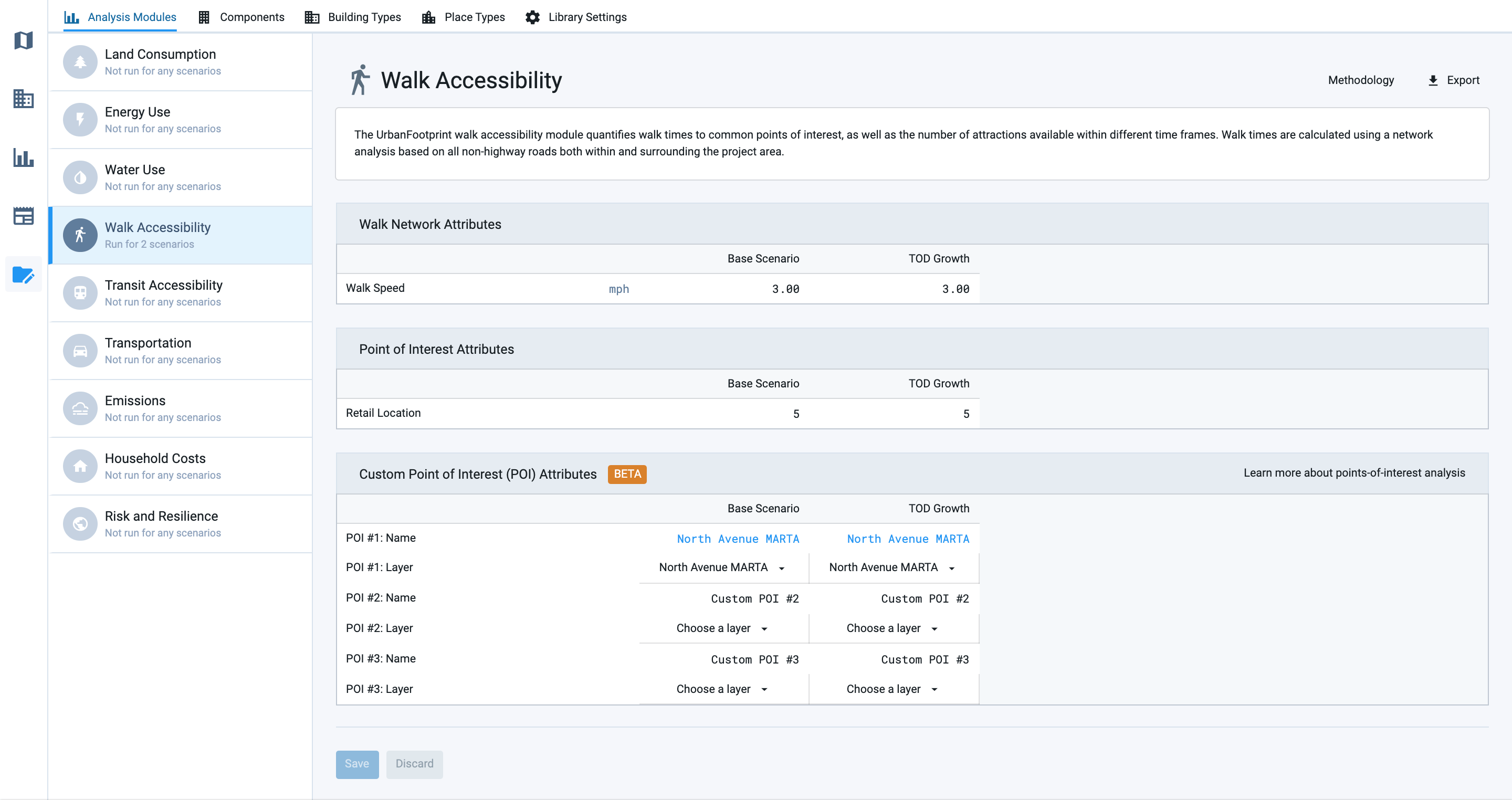
Setting custom points of interest in Manage mode
Click Save to save your edits.
Run the Walk Accessibility module. From Analyze mode, run the Walk Accessibility module for the scenario(s) for which you specified the transit station and any other custom POIs. Changing the analysis parameters of a scenario renders any previous analysis as out of date, so if you ran the module previously you'll need to run it again to apply the new parameters.
Map the accessibility results. We'll first look at the outputs on the map. Activate the Walk Access to Destinations layer and select the custom POI column for the transit station. Ours is called "Custom POI #1: North Avenue MARTA - Time to Nearest." You can edit the layer symbology to adjust the classes and colors displayed.
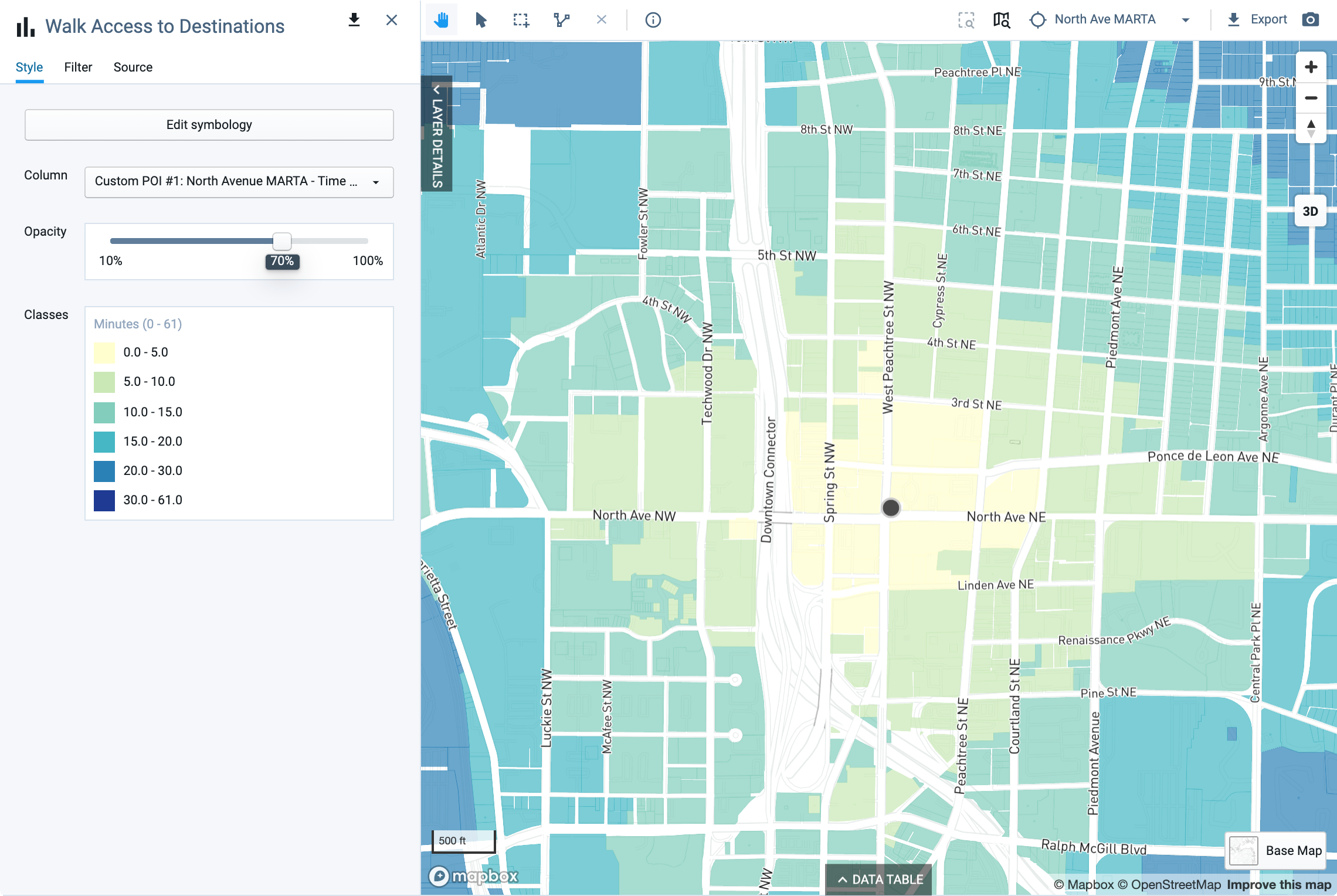
Viewing the custom POI walk access outputs
Create a walkshed layer. We can now create a standalone layer to represent the 10-minute walkshed around the station.
Click the Filter tab for the Walk Access to Destinations layer.
Add a filter for the custom POI output column (in this case, "Custom POI #1: North Avenue MARTA - Time to Nearest") and specify an access range, in minutes. We'll select all parcels within a 0 to 10 minute walk of the station.
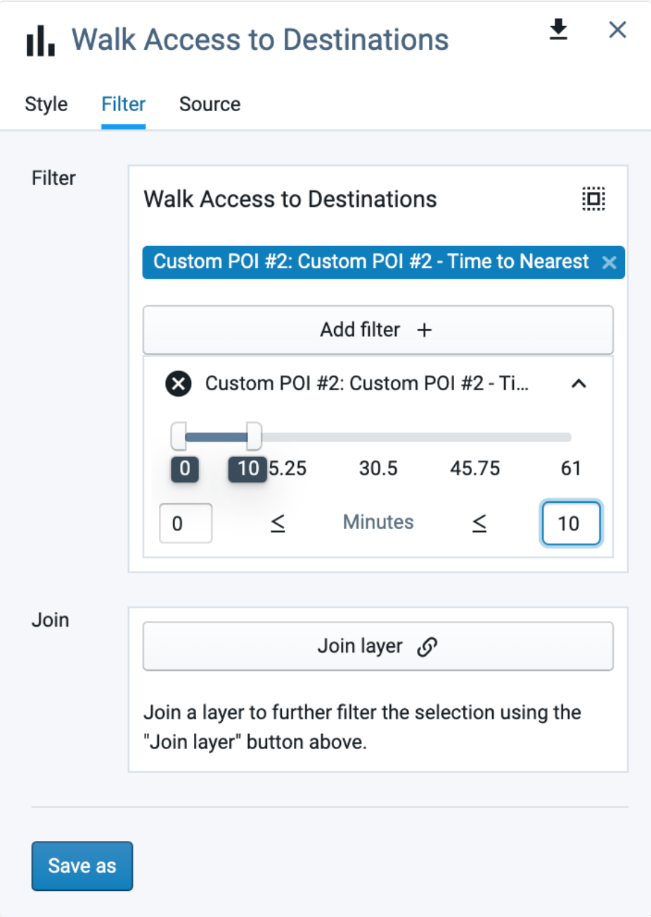
Filtering the Walk Access to Destinations output to save as aw
Click Save as to save the filtered selection as a layer. We'll call it "North Avenue MARTA: 10-minute walkshed." You can now map this layer on its own, and use it in join filters with other layers. The map below shows the 10-minute walkshed with a half-mile buffer around the station layered on for reference.
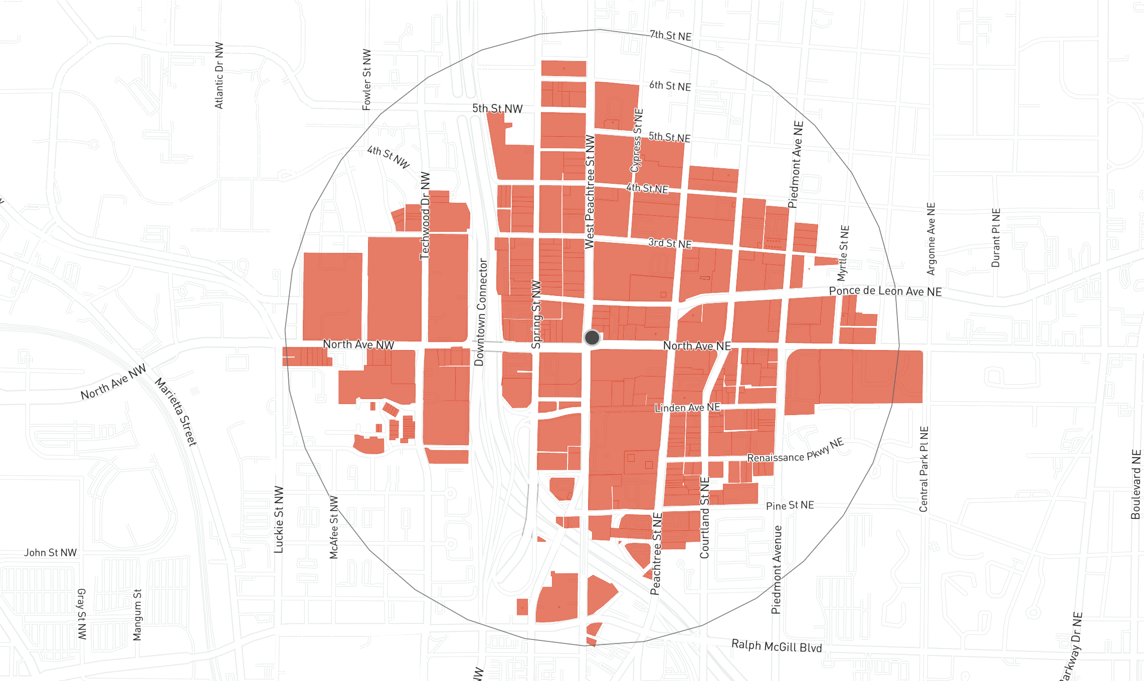
Ten-minute walkshed saved as a filtered selection from the Walk Access to Destinations output layer
Join the walkshed layer to the Base Canvas. Now, we'll select all parcels in the Base Canvas that fall within the 10-minute walkshed. Joining the walkshed to the Base Canvas will allow you to evaluate housing, jobs, and existing land uses in the area.
Select the Base Canvas to activate it and view it on the map.
Click the Filter tab.
Click Join layer, then select the filtered layer that you created in Step 6. All the matching features from the Base Canvas will be selected.
Click Save as to save the walkshed selection as a new layer. Now, you can map the walkshed around the station according to any Base Canvas attributes, as shown below.

Base Canvas land use in the 10-minute walkshed of MARTA's North Avenue Station
View and/or export the data table for the walkshed selection. If you export the data table, you can summarize the data in various ways, for example by land use type.
Join the walkshed with other layers for further analysis. Just as you joined the walkshed layer to the Base Canvas, you can join it to any other layers as relevant for your work—for example, a scenario canvas to select features to be painted; the Parcel Reference Data layer to assess current property values or redevelopment potential; or layers for places of interest, such as bike stations.
The example below shows improvement-to-land value ratios (low values for which can indicate underutilization and redevelopment potential) for residential and commercial parcels in the walkshed of the North Avenue MARTA station.
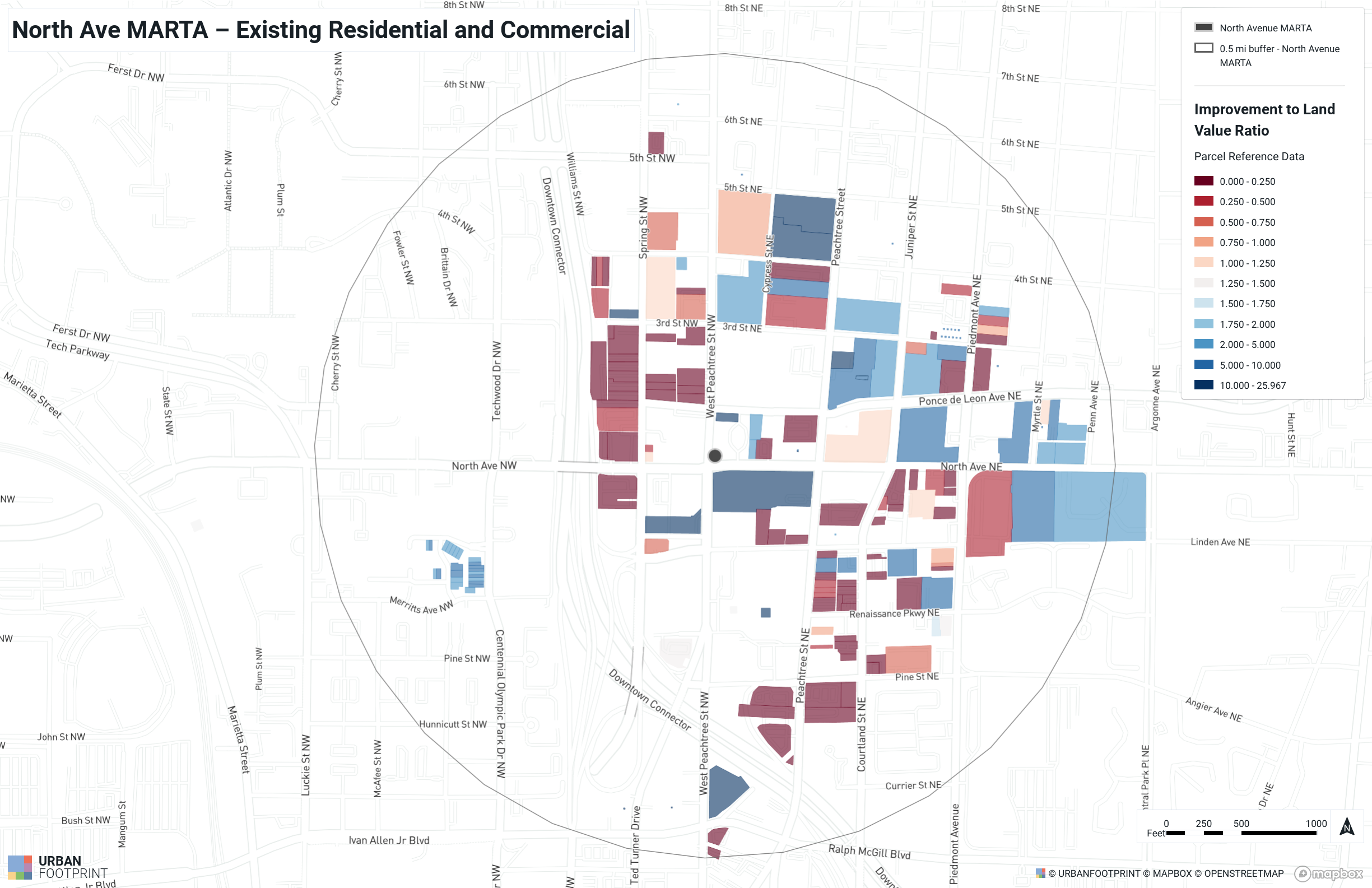
Assessing redevelopment potential by joining the walkshed to the Parcel Reference Data layer
Identify Gaps in Access to Critical Community Facilities
Custom POI accessibility analysis can be used to identify where residents have poor access to facilities critical for public safety, and assess how new locations could address those gaps. In this example, we'll analyze transit access to cooling centers, which are important to safety during heat waves.
Upload a point layer reflecting facility locations. Since they are subject to change, data for cooling center locations need to be sourced or developed locally. Upload by clicking the Upload Layer button
 in the upper right portion of the Layers pane. See Upload Data Layers for details on uploading layers. For our example, we'll upload a layer of community centers that serve as cooling centers in Fresno, California.
Navigate to the Transit Accessibility module inputs in Manage mode.
Enter Manage mode by clicking the Manage mode button
in the Mode bar.Click the Analysis Modules tab, if it is not active already.
Select the Transit Accessibility module from the list on the left.
Enter parameters for the custom POIs. Find the input parameters in the Custom Point of Interest Attributes parameter section, as shown below. We'll enter parameters for the Base Scenario.
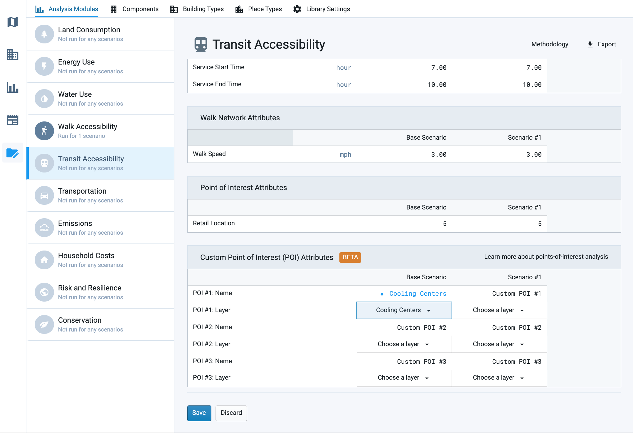
Enter a name for the cooling center POIs. POI names appear in the headers of the results charts, and in the column names of the analysis output layer. Double-click on the default name (e.g., "Custom POI #1") to edit it. We'll enter "Cooling Centers."
Select the layer containing the cooling centers. The drop-down list allows you to select from the point layers loaded to your project. Find the layer that you added. Ours is called "Cooling Centers."
Click Save to save your edits.
Run the Transit Accessibility module. From Analyze mode, run the Transit Accessibility module for the Base Canvas. Changing the analysis parameters of a scenario renders any previous analysis as out of date, so if you ran the module previously you'll need to run it again to apply the new parameters.
Map the cooling center accessibility results. Activate the Transit Access to Destinations layer and select the custom POI column for the cooling centers. Ours is called "Custom POI #1: Cooling Centers - Time to Nearest."
The map below uses the default symbology for custom POI outputs. You can edit the layer symbology to adjust the classes and colors displayed.
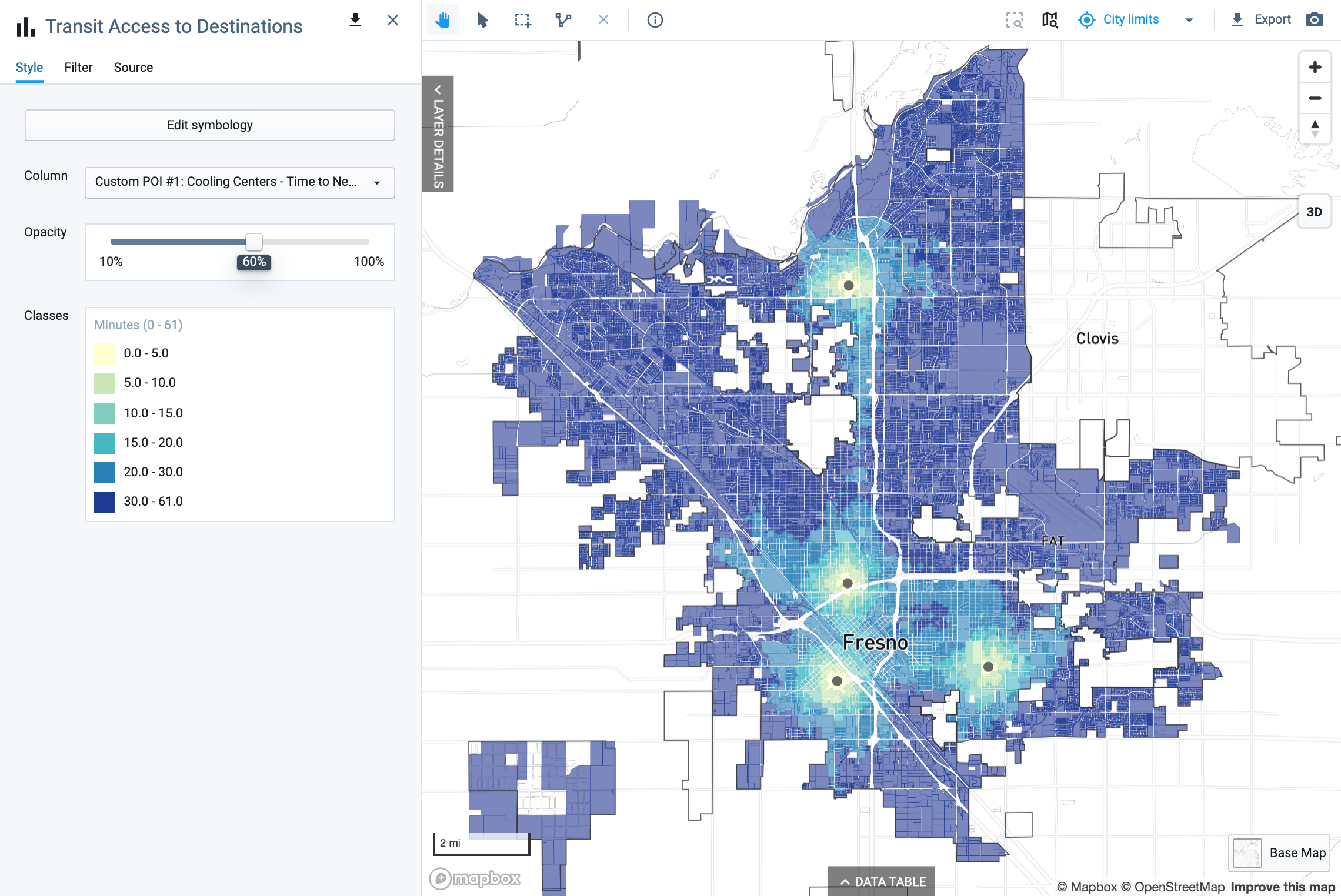
Viewing the cooling center transit access outputs
From the map, we can see many access gaps—areas where residents must travel over 30 minutes by transit to reach a cooling center.
View the cooling center accessibility results chart. In the Analysis pane, you can find the summary chart indicating the percentage of residents in the project area within a 10, 20, or 30 minute combined transit/walk trip to a cooling center. We can see that roughly a quarter of Fresno residents can reach a cooling center within 30 minutes, while the rest must travel longer.
Use the data table to quantify population by access range. The Transit Access to Destinations layer contains population counts for each canvas feature. You can apply a filter on the cooling center POI output column to select parcels and associated population in areas with and without reasonable access to cooling centers.
Click the Filter tab for the Transit Access to Destinations layer.
Click Add filter +, then select the custom POI output column (in this case, "Custom POI #1: Cooling Centers - Time to Nearest") and specify an access range, in minutes. We'll select all parcels from which it takes over 30 minutes to reach the nearest cooling center.
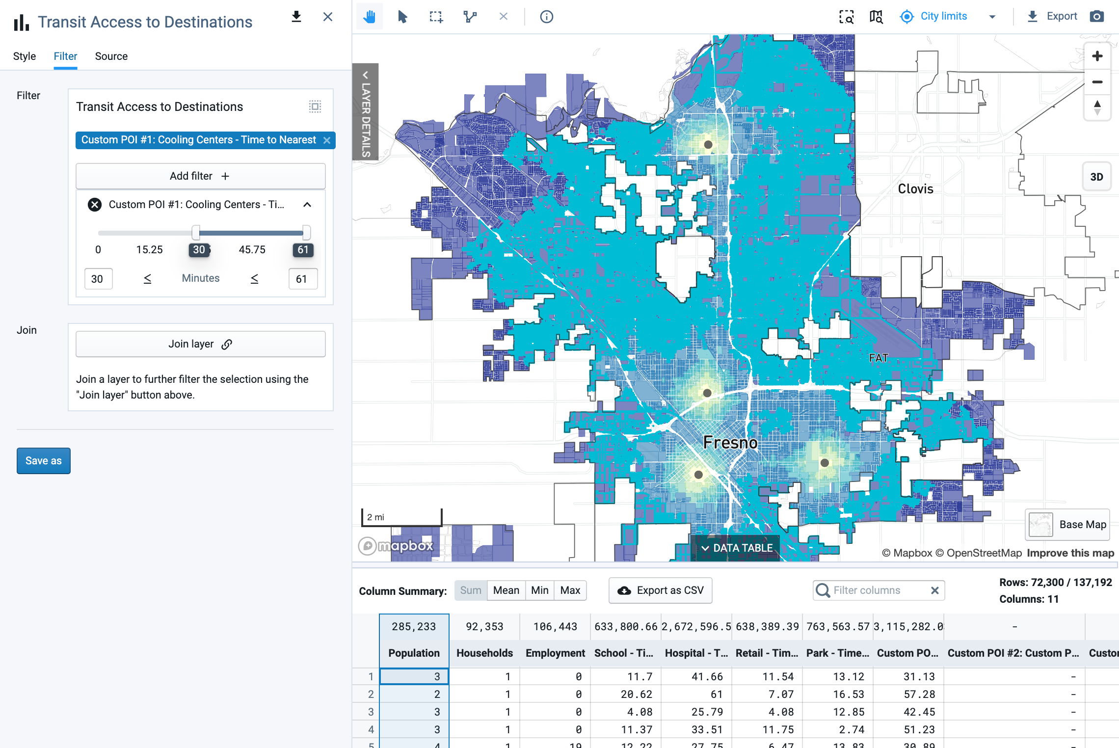
Using a filter to select parcels within a 30-minute trip to a cooling center
View the data table for the summarized result. The column summary for the "Population" column can show the sum total within the selected parcels. We can see that over 285,000 residents cannot reach a cooling center within 30 minutes—more are needed.
Identify the location of vulnerable residents. In planning for additional sites, it's important to understand where residents may be most vulnerable to extreme heat. Risk factors include poverty; age; underlying health conditions; lack of access to vehicles; limited English proficiency; impervious surfaces; particulate matter concentrations; and more. We'll explore where vulnerable populations lack cooling center access by bringing in reference data.
From the Layer Manager, add the Heat Wave Vulnerability Index - California (CHAT) layer. The California Heat Assessment Tool (CHAT) developed for California state agencies incorporates a range of risk factors correlated with negative health outcomes into an index score by census tract. The CHAT Heat Health Action Index data is available as a reference data layer. If you're working outside California, you could use other socio-demographic layers indicative of vulnerability, such as percentage elderly population from the Census Planning Database.
Classify the Heat Health Action Index column using quantiles. For this example, we'll classify the index scores using quartiles (four quantiles). This tells us that the top quartile of census tracts in Fresno have an index score of 52.6 and above.
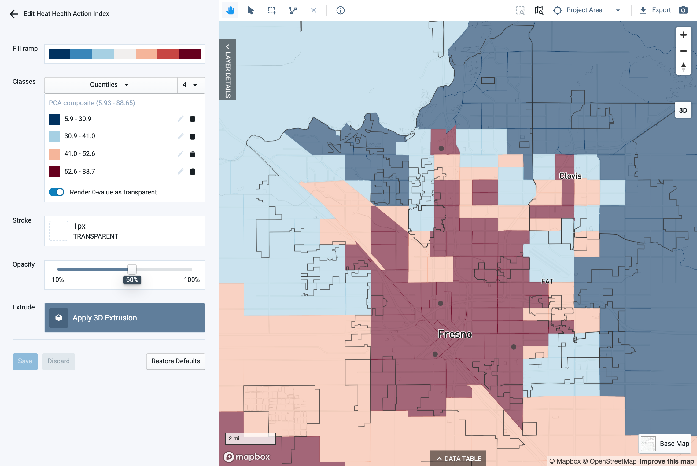
Classifying the CHAT Heat Health Action Index data
Locate vulnerable population with low access to cooling centers. To locate population with high vulnerability and low access to cooling centers, we'll select features from the Transit Access to Destinations layer using a filter and a join to the Heat Wave Vulnerability Index - California (CHAT) layer.
Click the Filter tab for the Transit Access to Destinations layer.
Click Add filter +, then select the custom POI output column (in this case, "Custom POI #1: Cooling Centers - Time to Nearest") and specify an access range, in minutes. Again, we'll select all parcels from which it takes over 30 minutes to reach the nearest cooling center. This is the same selection that we made earlier, so it may still be active.
Click Join layer, then select the Heat Wave Vulnerability Index - California (CHAT) layer.
Click Add filter + for the join layer, then select the Health Health Action Index column. Specify the range for the top quartile as identified by the data classification in step 7. For Fresno, this range is 52.6 and above.
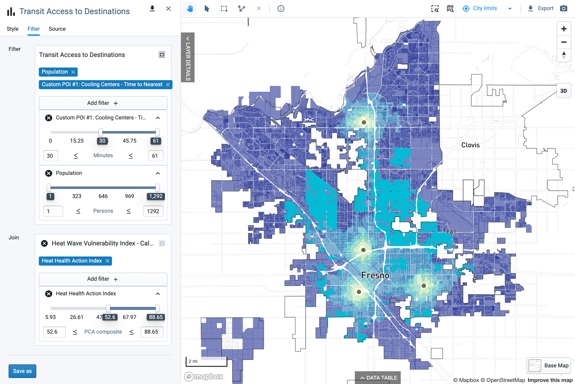
Applying a filter and join to select parcels with low cooling center access in high-vulnerability census tracts
Click Save as to save the selection as a new layer. We'll call this layer "Transit Access to Cooling Centers > 30 min; CHAT index top quartile."
Map and quantify vulnerable population with low access to cooling centers. With your filtered layer now created, you can cleanly map the areas where residents are most vulnerable to heat, yet have low access to cooling centers.
Map the saved filtered layer, "Transit Access to Cooling Centers > 30 min; CHAT index top quartile."
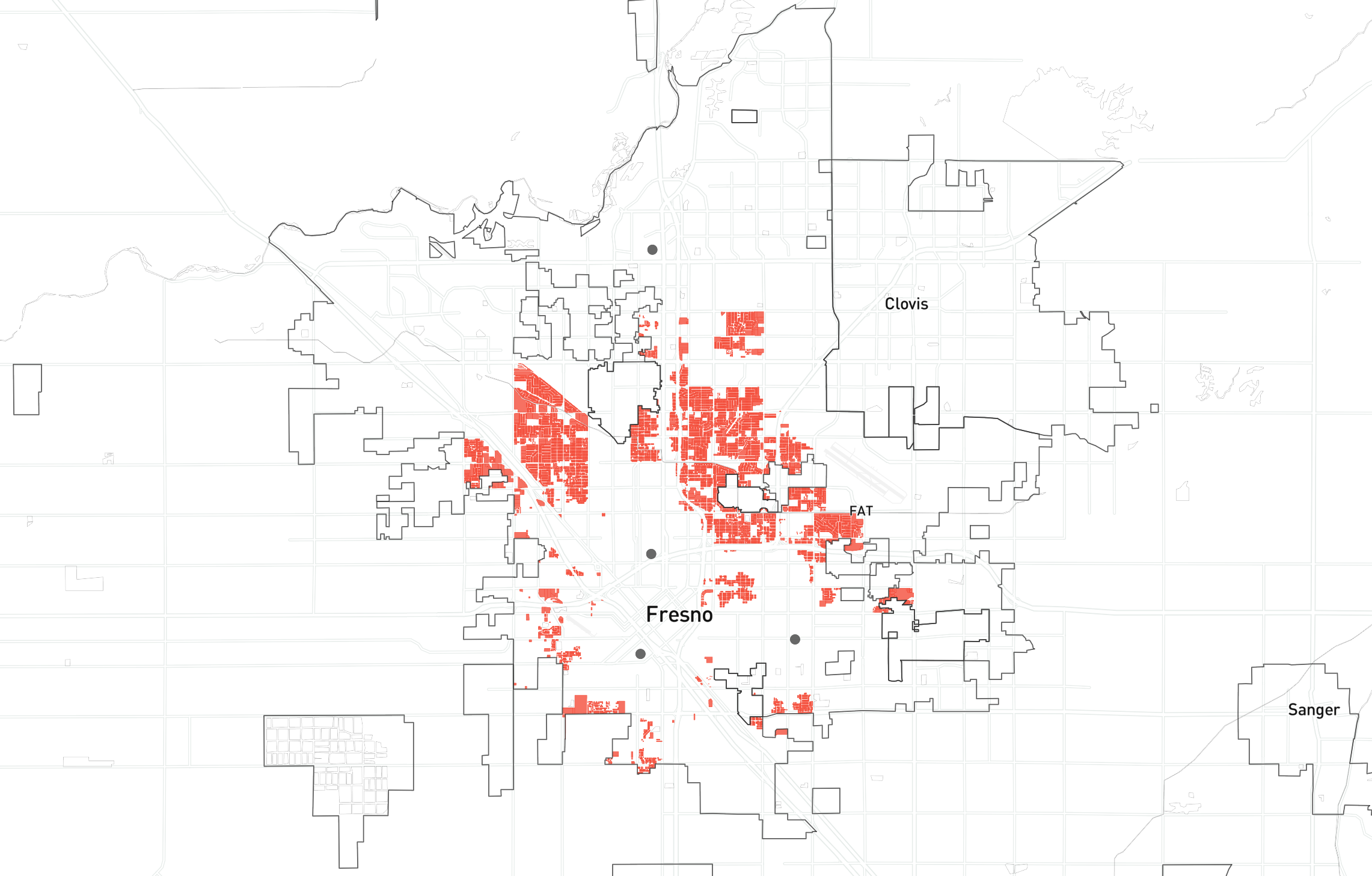
Parcels where residents have low access to cooling centers and high vulnerability to heat waves
View the data table for a summarized result. The column summary for the Population column can show the sum total within the selected parcels. Now, we can see that there are approximately 124,000 residents in high-vulnerability census tracts who cannot reach a cooling center within 30 minutes.
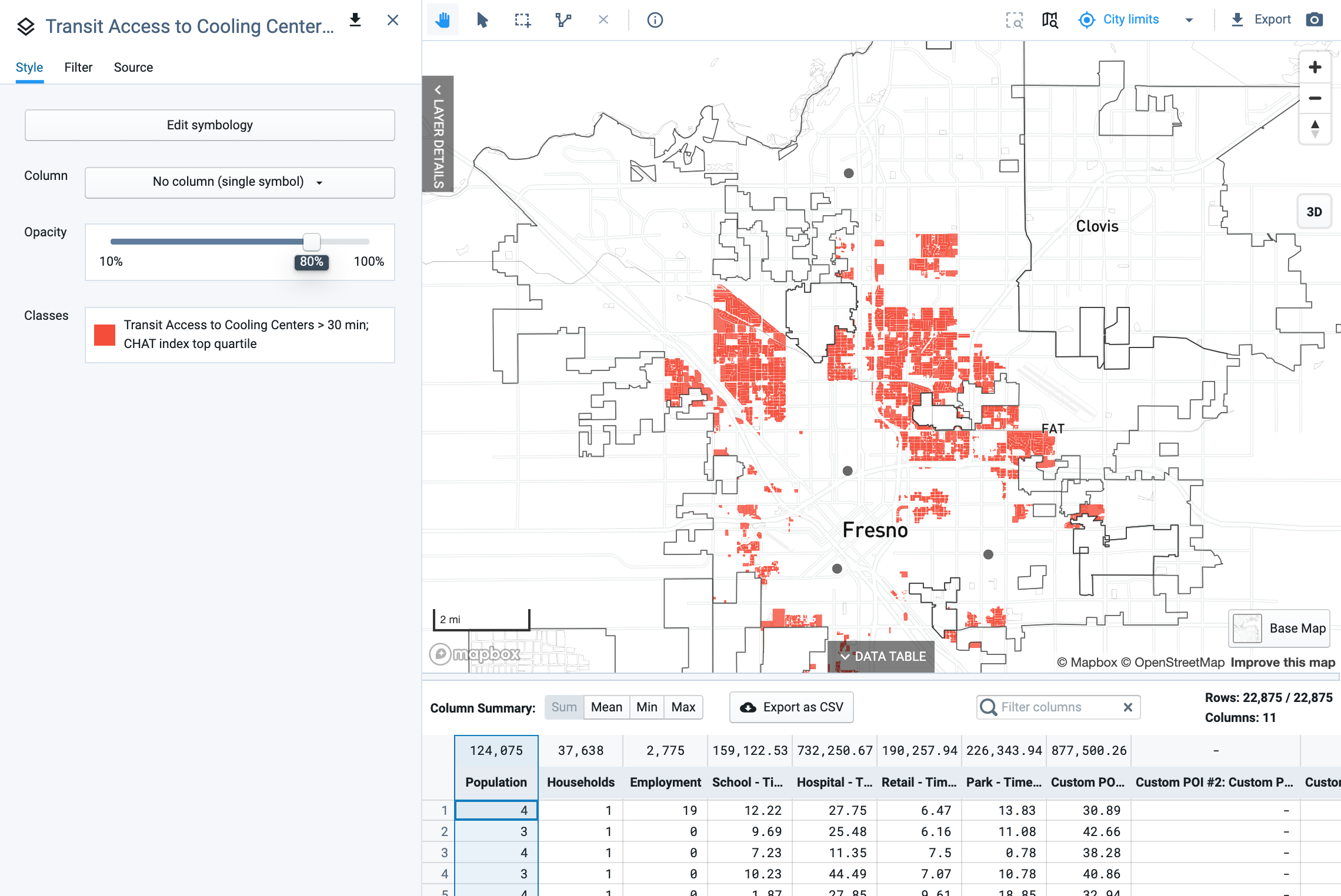
This analysis can guide the siting or designation of additional cooling center locations. Just as you measured access to existing locations, you can measure access to additional sites to assess how well they can serve to close critical gaps.
Create Custom Layers in GeoJSON Format
Creating GeoJSON files at geojson.io is convenient for quickly creating spatial data for use in Analyst. Standalone GIS software is not required. You can use the tool to create polygon layers to use as custom project boundaries, or point layers for use in custom point of interest (POI) accessibility analysis. You can also create or edit spatial data layers to upload to the platform for general use.
From your web browser, go to geojson.io. The site opens with a map view on the left, and a data/information panel on the right. For help in using the tool, you can see the Help tab in the panel on the right.
Navigate to a location. Click on the Search icon at the upper right and enter the name of a place, a street, or an address. You'll be able to select your intended location from the drop-down list. Pan and zoom as needed to focus on the area where you'll be creating features.
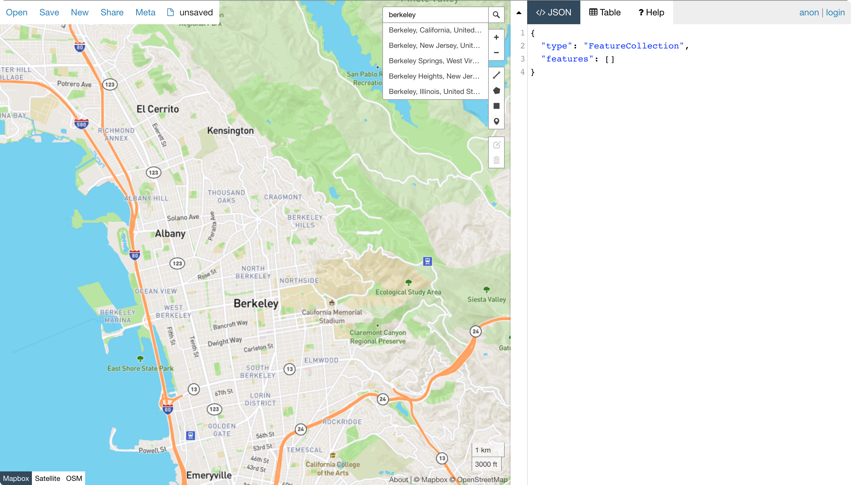
Create features. You can create polyline, polygon, rectangle, or point features using the drawing tools in the toolbar. Select a tool, then draw on the map according to the geometry type.
With the point drawing tool, you can simply click on the map to create a point feature. With the polyline and polygon drawing tools, click on the map to set the vertices of your features. With the rectangle drawing tool, click and drag to draw a rectangle area.
Note that Analyst only handles layers containing a single geometry type. For example, you can upload a layer containing points, but not one containing a combination of points and lines.
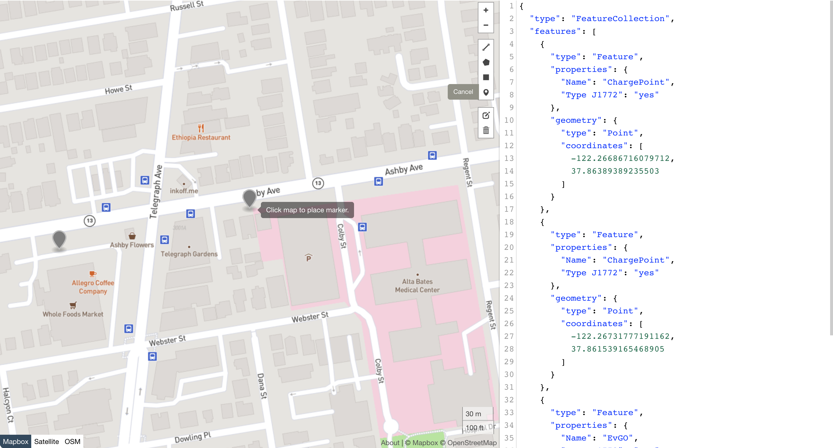
Creating a new point feature
Add attribute data. You can enter attribute data for each feature in a table that appears when you click on a feature. Click the + Add row button and enter a column name on the left, and a value on the right. Alternatively, you can click the Table tab in the panel on the right to enter information directly in the data table.
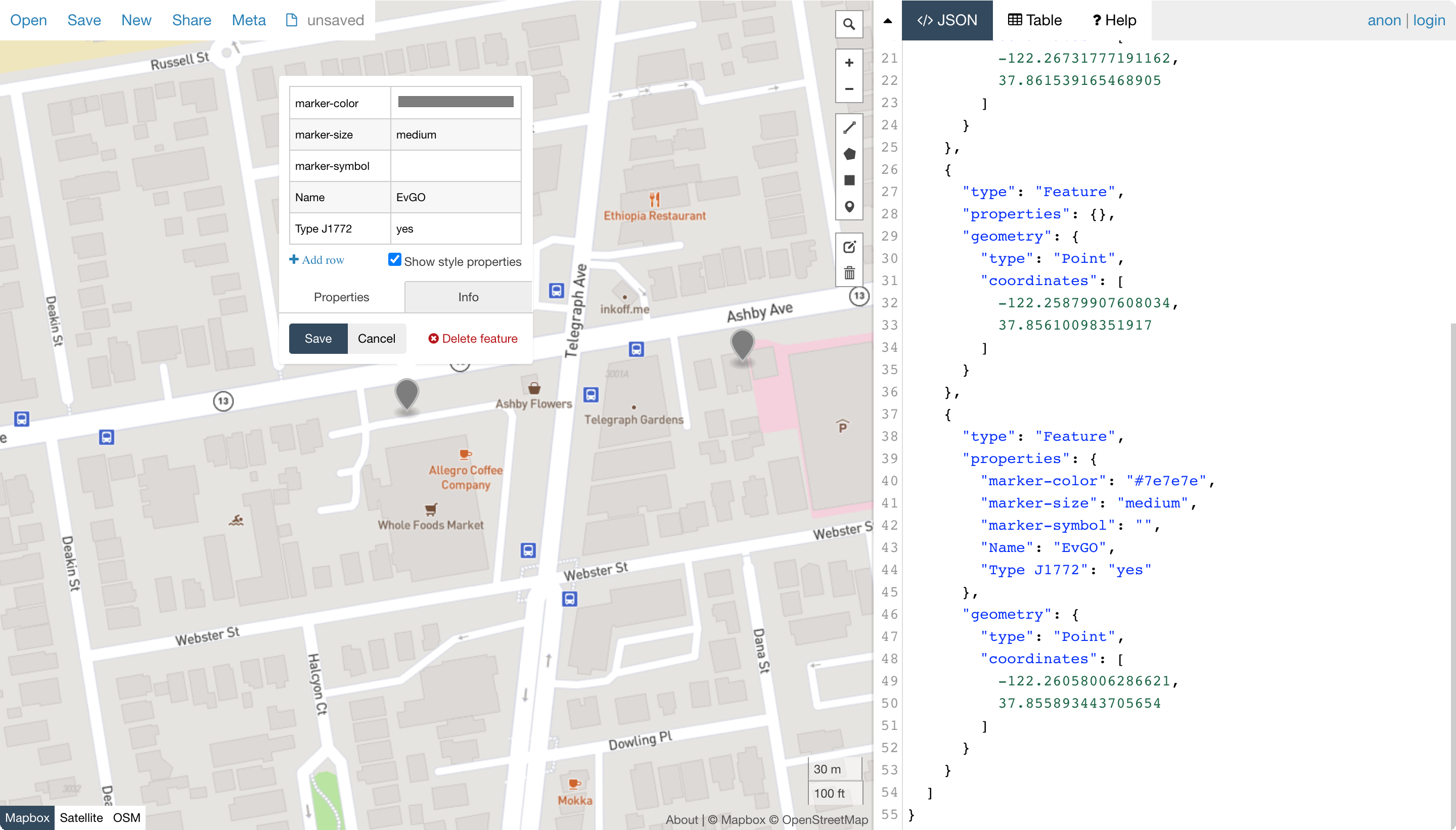
Entering attribute data for an individual feature
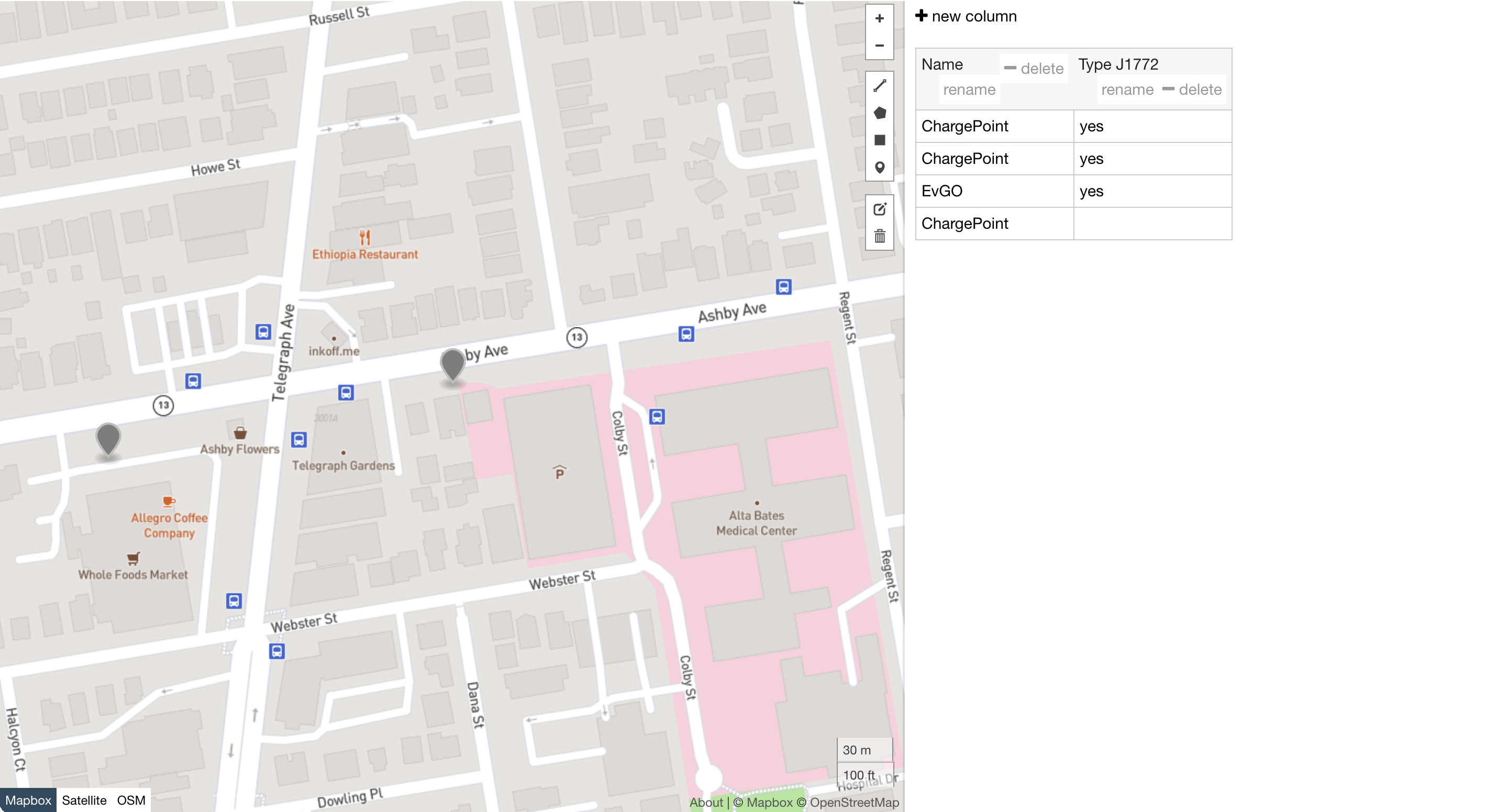
Entering attribute data using the data table
Save your data layer. Once you've finished drawing features and entering attribute data, you can save as a GeoJSON file. From the Save menu at the upper right, select GeoJSON (note that other formats are available). The GeoJSON file will be automatically downloaded to your computer.
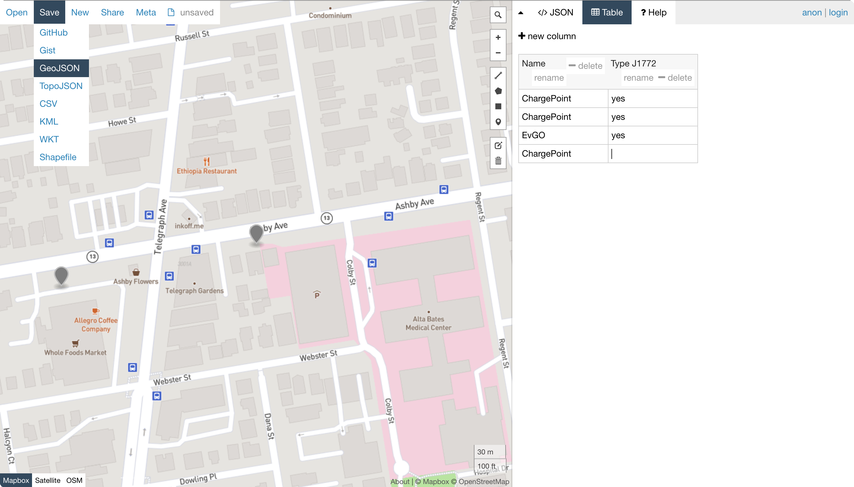
Saving your data as a GeoJSON file
Rename the GeoJSON file. The downloaded file will be given a generic name such as "map.geojson." Rename the file so you can identify it later.
Upload your GeoJSON data to Analyst. Now, you can upload your new data for use in Analyst. See Upload Data Layers for guidance.