Reporting
 |
From maps and charts to data exports, Analyst provides what you need to present existing conditions assessments and scenario metrics. The tutorials in this section take you through Report mode and features for presenting the essentials of your scenario work.
Compare Scenario Summary Statistics
Analyst uses a set of "summary statistics" to represent development characteristics across scenarios. Summary statistics include totals for population, households, homes, jobs, and building area. Whether you're developing scenarios to meet control totals for growth, or to compare the capacity of plans or development options, summary statistics are useful for checking progress as you develop scenarios, and reporting final results. In this tutorial, we'll view, compare, and export summary statistics for three scenarios.
Data Layers | Features |
Scenarios |
Enter Report mode and view Summary Statistics. Click the Report mode button
 in the Mode bar. If not already selected, select Summary Statistics from the list on the left side of the screen.
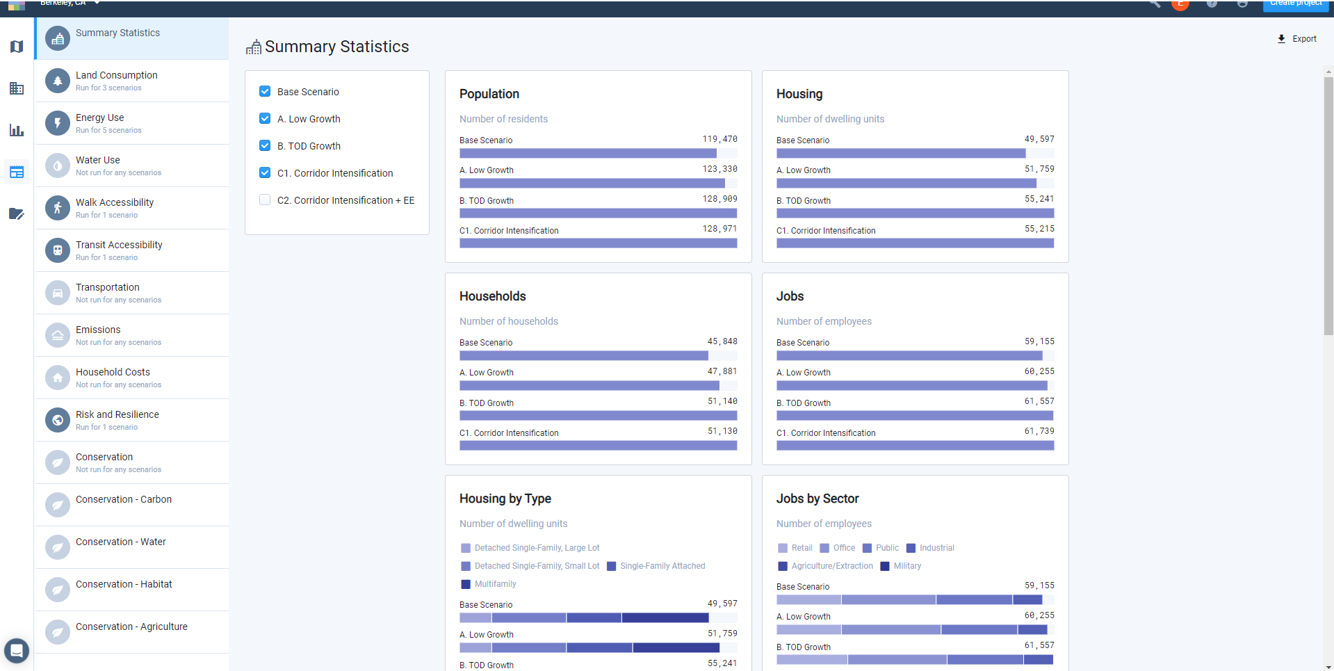
Select scenarios to compare. Use the scenario checkbox controls in the upper left corner to select the scenarios for which you would like to view statistics. By default, all scenarios are turned on. For our example, we'll look at three scenarios for our project area: Low Growth, TOD Growth, and Corridor Intensification. (We've also created a fourth scenario that includes the same land use as the Corridor Intensification scenario, but with different module parameters for the Energy Use module to represent improvements in building energy efficiency. We'll look at this in the next tutorial.)
Scenario Summary Statistics
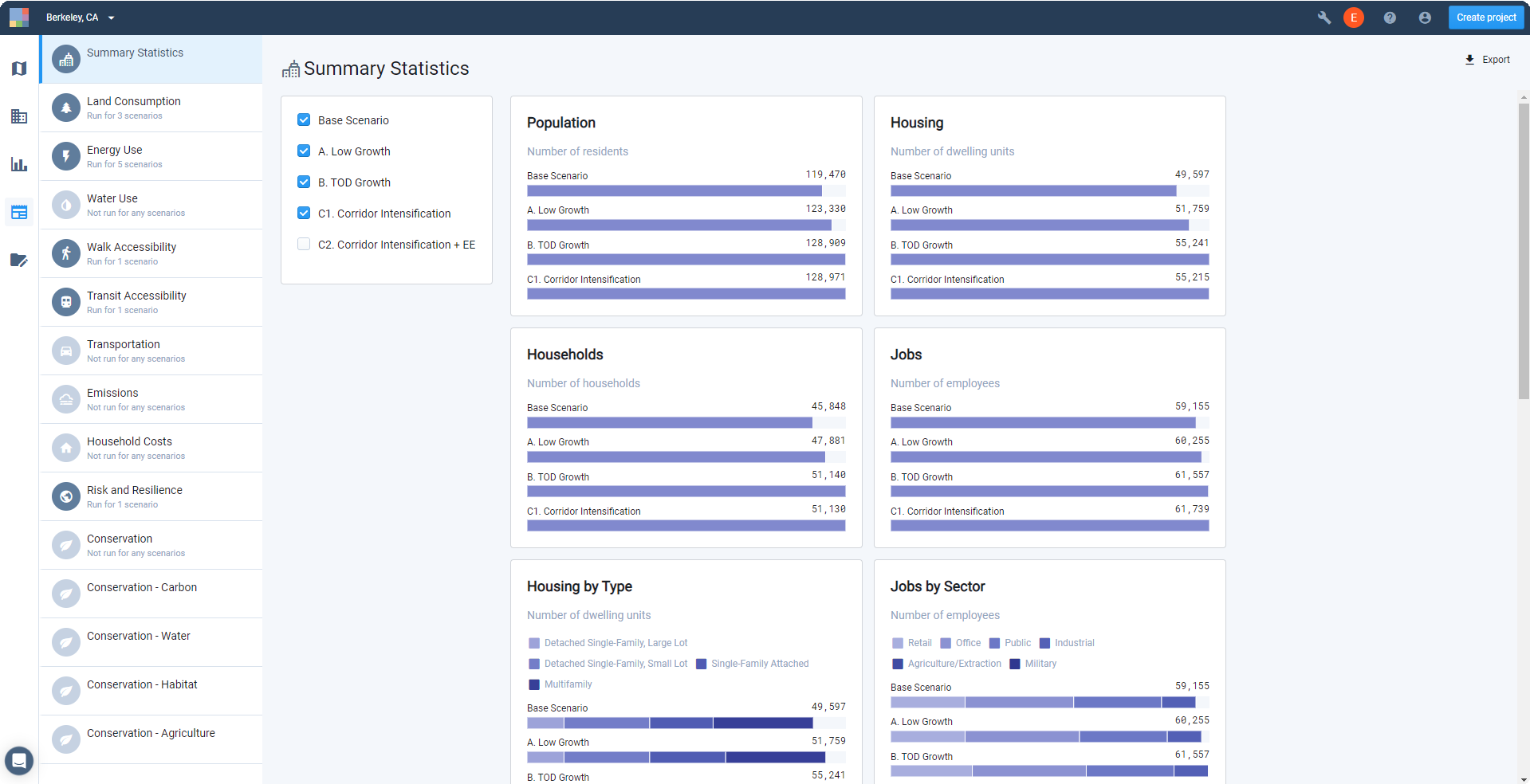
View and compare scenario statistics. Scroll down in the Summary Statistics screen to see all the charts. They include:
Population
Housing
Households
Jobs
Dwelling units by type
Single-family detached, large lot
Single-family detached, small lot
Single-family attached
Multifamily
Jobs by sector
Retail
Office
Public
Industrial
Agriculture/Extraction
Military
Residential building floor area by housing type
Detached Single-Family, Large Lot
Detached Single-Family, Small Lot
Single-Family Attached
Multifamily
Retail building floor area by subsector
Retail services
Restaurant
Arts & entertainment
Accommodation
Other Retail Building Area
Office building floor area by subsector
Office services
Medical services
Public building floor area by subsector
Public administration
Education
Industrial building floor area by subsector
Transportation/Warehouse
Wholesale
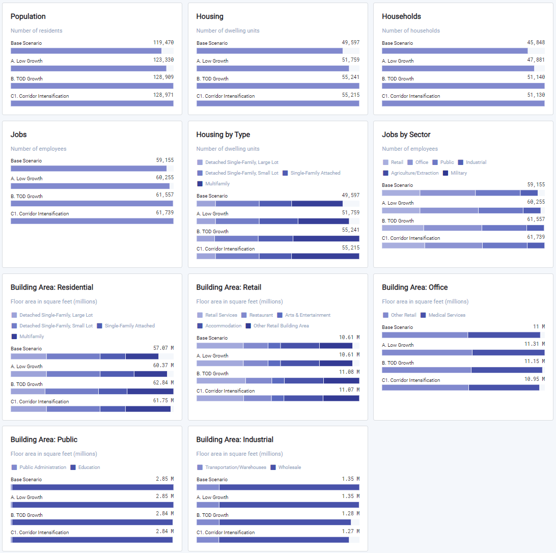
Scenario Summary Statistics charts
For our example scenarios, we can see that the TOD Growth and Corridor Intensification scenarios have been built to meet approximately the same amount of population, household, and employment growth. They differ in the mix of housing types and distribution of employment by sector, as indicated by the Housing by Type and Jobs by Sector charts. (Hovering over the individual sections of stacked bar charts displays sub-category values.) Lastly, we can see variations in the amount of building area required to accommodate the growth, in total and by housing or commercial space type.
The charts are dynamically generated and cannot be downloaded. However, you can export the summary statistics to develop custom charts in other programs.
Export a Summary Statistics Report. Click the
 Export button. An Excel-format report containing all data as represented by the charts will be downloaded to your computer.
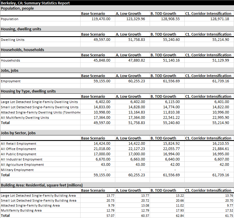
Partial view of Summary Statistics Report mode
Using the exported report, you can run further analysis—for example, calculating net growth relative to the Base Scenario—and create custom charts. The second tab in the workbook contains metadata including the project name, type of report, export date and time, and the names and descriptions of the included scenarios.
Compare Scenario Results
The Analyst analysis modules produce a range of outputs:
Comparative results for multiple scenarios, accessed via Report mode,
Output layers that can be examined on the map and in the data table via Explore mode, and
Summary results for individual scenarios, accessed via Analyze mode
In this tutorial, we'll view, compare, and export analysis module results via Report mode. For guidance on working with summary metrics and output layers for individual scenarios, see Work with Analysis Module Outputs.
Data Layers | Features |
None |
You'll need to run analysis modules for your scenarios before comparing results. For our example, we'll look at outputs from the Energy Use module.
Enter Report mode. Click the Report mode button
in the Mode bar. The Report screen appears, with the analysis modules listed at left beneath the option for Summary Statistics. The run status for each module is shown.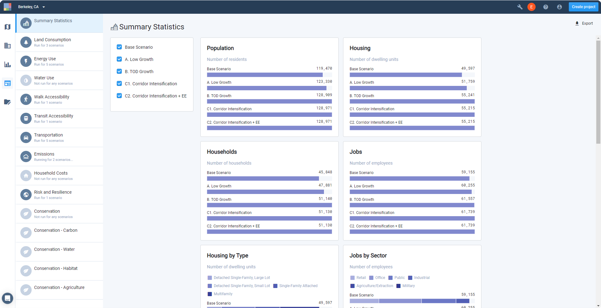
Default view of Report mode screen (note that the Conservation module is available in California only)
Select an analysis module. We'll select the Energy Use module.
Select scenarios to compare. Use the scenario checkbox controls in the upper left corner to select the scenarios for which you would like to view results. By default, all scenarios are turned on. For our example, we'll look at four scenarios for our project area: Low Growth, TOD Growth, and two variations of Corridor Intensification—C1 and C2 for short. C1 and C2 feature the same land use, but C2 uses different parameters for the Energy Use module to represent improved building energy efficiency.
Report Mode > Scenario Summary Statistics
View and compare summary results. Scroll down in the Energy Use report screen to see all the charts. The summary results include total annual energy use (combined electricity and natural gas), electricity use, and natural gas use for residential and commercial buildings; per-household annual energy use; annual residential energy costs (produced by the Household Costs module); and annual building energy GHG emissions (produced by the Emissions module).
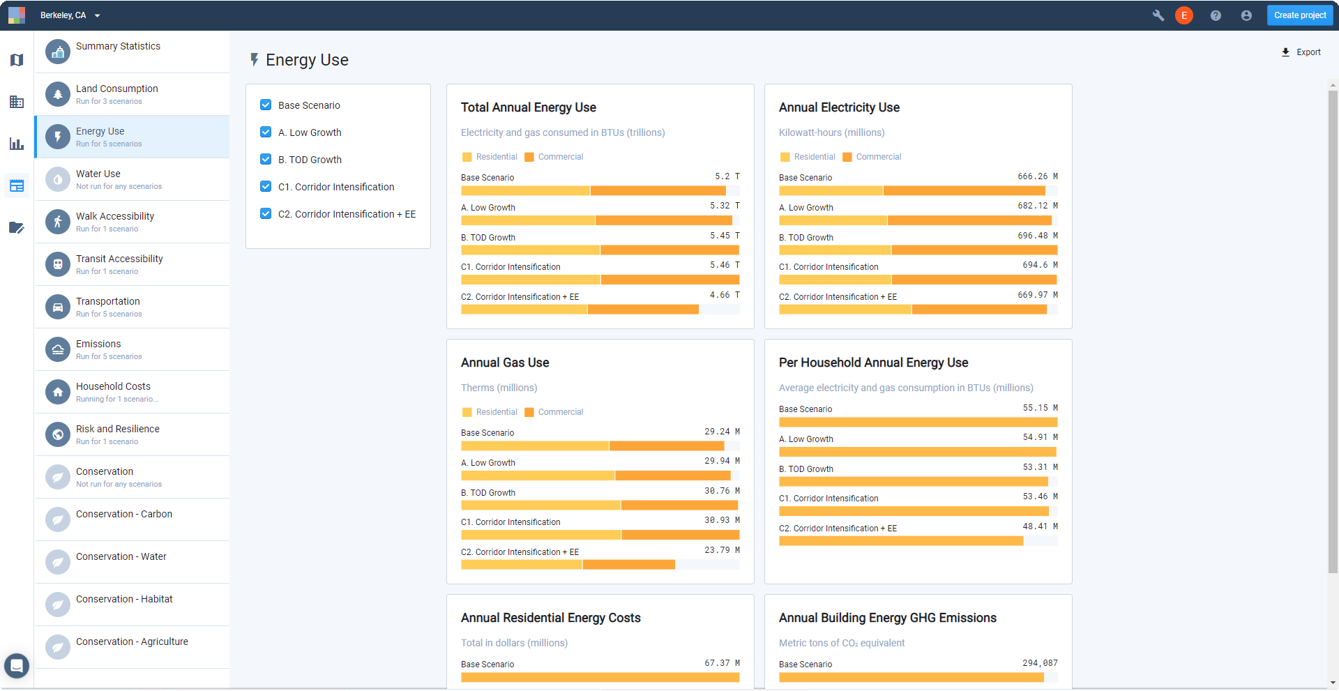
Energy Use report screen
The scenario-total and per-household metrics represent different options for presenting scenario results. In our example, the Low Growth scenario features lower housing and employment growth than the TOD Growth and Corridor Intensification scenarios (as seen in the Summary Statistics charts). For this reason, it might not be appropriate to compare energy use among the scenarios on the basis of scenario-wide annual totals. They might instead be compared on the basis of the per-household metrics.
For scenarios C1 and C2, which do not vary in land use, we can see differences in energy use, household costs, and GHG emissions that are attributable to improvements in energy efficiency alone.
Some summary metrics charts feature stacked bars. For the energy use results, the stacked bars are used to delineate results for residential and commercial buildings. Rolling over the individual sections displays sub-category values.
The charts created in Analyst are dynamically generated and cannot be downloaded. However, you can export the summary results to develop custom charts in other programs.
As another option, you can work directly with analysis module layers to extract more refined outputs, for example to summarize results for specific areas.
To export scenario results, click the Export button
. An Excel report containing all data as represented by the charts will be downloaded to your computer.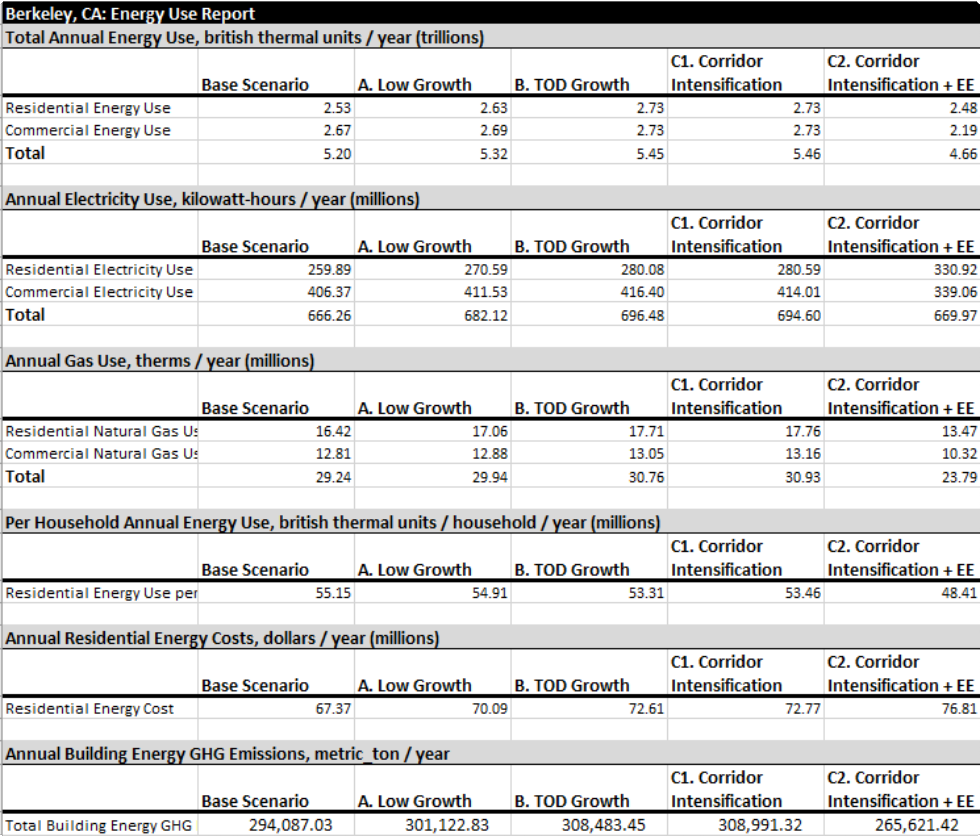
View of Energy Use Report export
Using the exported report, you can run further analysis—for example, calculating the differences among scenarios—and create custom charts. The second tab in the workbook contains metadata including the project name, type of report, export date and time, and the names and descriptions of the included scenarios.
Export Layer Data
Analyst allows you to export layer data to share or bring into other applications for advanced mapmaking or analysis. A number of export formats are available, including CSV (with or without geometry information), GeoJSON, GeoPackage, shapefile, and Scalable Vector Graphics (SVG). You can export data for most layers, including reference data layers, the base canvas, scenarios, analysis outputs, and filtered layers. The only exceptions are for data with source restrictions.
In this tutorial, we'll export a layer first as a shapefile, then as an SVG file.
Data Layers | Features |
Any layer to be exported |
Select a layer. From Explore, Build, or Analyze mode, click on a layer in the Layers List. For our first example, we'll work with the Parks & Open Space reference data layer.
Create a filtered layer to include only the features you'd like to export. Layer Export will, by default, export the entirety of a layer, even if a filter selection is active. Exports also include features, if any, that are beyond the boundaries of your project and context areas. If you want to restrict your export to features within your project area alone, you can first create a selection and save it as a filtered layer.
Click the Filter tab for the Parks & Open Space layer.
Click Join layer, then select the Project Area layer.
Click Save as and give the filtered layer a name and a description, if desired.
Export the filtered layer as a shapefile. From the Layer Details pane, click the Download layer button
and select the shapefile format from the list. The available formats include:Comma-separated value (CSV) with geometries – A tabular data format that includes a geometry key that specifies feature locations. CSVs with geometries can be imported into GIS and mapping tools.
CSV without geometries – A tabular data format, suitable for use in spreadsheet or database applications.
GeoJSON – An open standard format for storing geospatial data.
GeoPackage – An open standard, compact format for storing geospatial data.
Shapefile – A geospatial vector data format for use in GIS programs. The layer is downloaded as a zip folder containing the shapefile (.shp) and supporting files.
Scalable Vector Graphics (SVG) – A vector graphics format for use in graphics programs such as Illustrator.
All spatial data exports from Analyst use the WGS84 projection, while the user interface, SVG exports, and map exports use the Web Mercator projection.
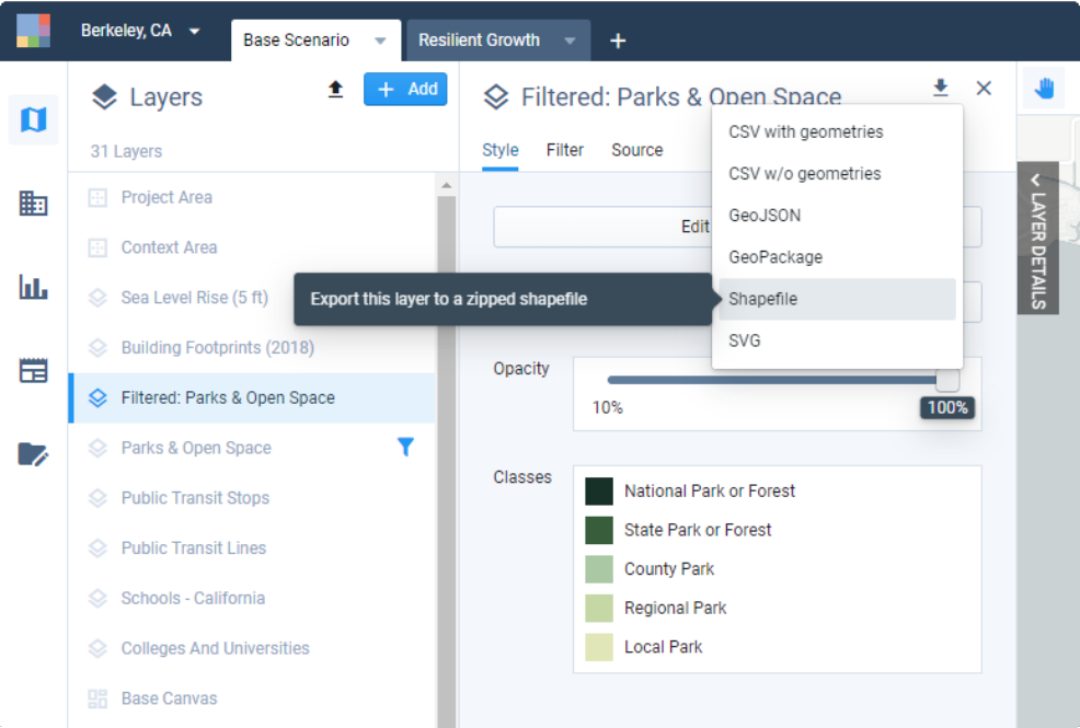
Layer export format selection
Analyst will prepare the data download, and a pop-up window will appear at the bottom of your screen when the layer is ready.
Note
If the download options are disabled, the selected layer is subject to export restrictions. Parcel Reference Data is limited to use within Analyst, while the Base Canvas data is restricted for a small number of counties, in accordance with source data restrictions.
Download your export. Click DOWNLOAD in the pop-up notification to download your data. The layer will be downloaded to your computer. Depending on their size, layer exports may take some time to download.
You can find the downloaded file in your default downloads folder, named according to your project and layer names. Shapefiles are exported as .zip files.
Export the filtered layer as an SVG file. Now, we'll export to SVG format. To support mapmaking in Illustrator and other graphics programs, SVG exports contain vector features grouped by class. With the Parks & Open Space layer, this means that we can export features grouped by Park Type. Analyst uses the currently mapped column (the column selected in the Style tab) as the basis for grouping features. While the data classes are maintained, fill and stroke styling are not.
If not already selected, select the Park Type column in the Style tab.
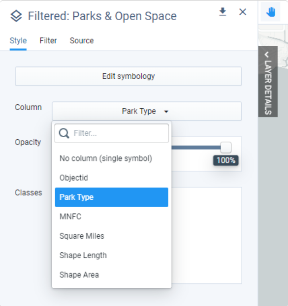
Selecting a column to determine SVG feature grouping
Click the Download layer
button and select the SVG format from the list. Analyst will prepare the data download, and a pop-up window will appear at the bottom of your screen when the layer is ready.
Download your export. Click DOWNLOAD in the pop-up notification to download your data. The layer will be downloaded to your computer. Depending on their size, layer exports may take some time to download.
You can find the downloaded file in your default downloads folder, named according to the project and layer names.
Open the SVG file in Illustrator. For our example, we'll look at the contents of the SVG file in Illustrator. If you use Illustrator, follow along and open the file.
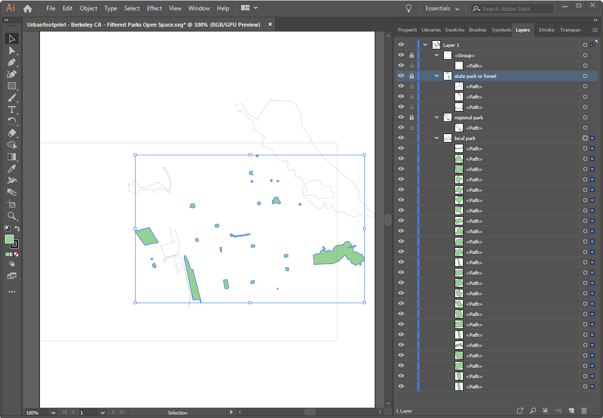
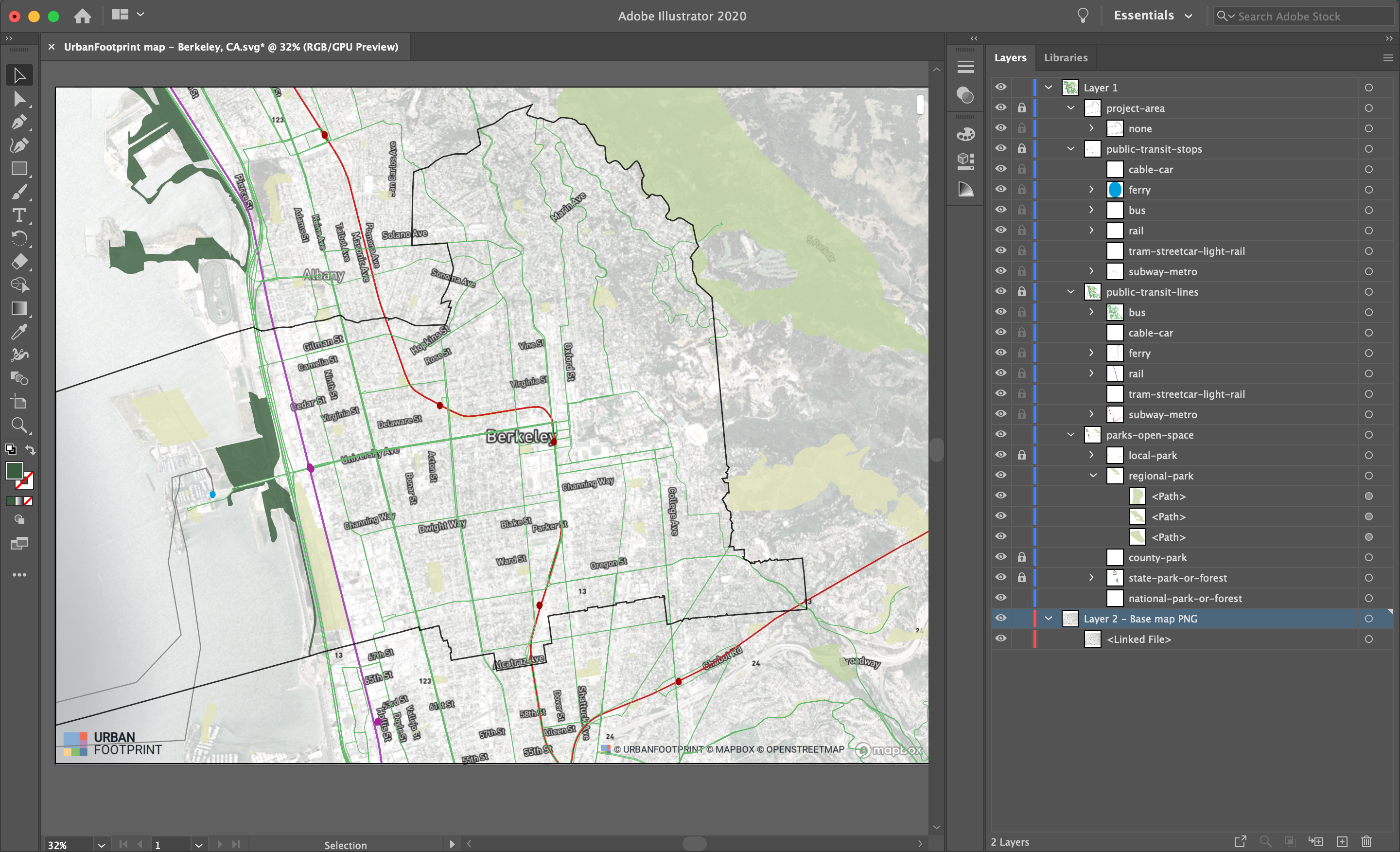
Parks & Open Space layer SVG export in Illustrator
Take note of a few elements:
Default style properties All objects come through with a white fill and black outline.
Project area extent. The rectangular area included in the topmost group corresponds to the outer extents of the project area. This is included as a reference point for aligning multiple vector layers.
Grouped features. The Layers panel shows the vector objects grouped by class -- in this case, the park types. Here, we've selected all the "Local Park" objects and given them a fill color.
SVG layer exports provide flexibility for custom mapmaking, and the creation of graphics incorporating geographic features.
Export Maps to SVG
Using the Map Export feature, you can export maps to scalable vector graphics (SVG) format for mapmaking with full design control in Adobe Illustrator or other vector graphics editing programs. An SVG vector map export is a single file that contains all map layers, symbolized and at the same extent as they appear in the map export view. From there, you can style features and add annotations and other map elements to produce map layouts just as you like. And finally, you can export your maps from SVG to PDF format for printing and sharing.
To produce a full map layout in Analyst, including a title, legend, north arrow, scale bar, and logo, you can export directly to a PNG image file instead. For more information, see Export a Map to PNG.
You can also export single layers to SVG format, as described in Export Layer Data, to produce files that contain all features for the entirety of your project area.
In this tutorial, we'll export a map as an SVG file, then look at its contents in Illustrator.
Data Layers | Any layers displayed in map view |
Features |
Style your map as desired. To support graphics handling in Illustrator and other programs, SVG exports include vector features grouped by layer and class. Analyst uses the currently mapped column (the column selected in the Style tab) as the basis for grouping features. The data classes are maintained as specified, as are fill and stroke styling.
Layer features that appear in the map are cropped to the rectangular extent shown in the map layout view. You'll have the opportunity to fine-tune the map layout view later.
Click the
Export button that appears above the top right corner of the map. The Export button is accessible from Explore, Build, or Analyze modes.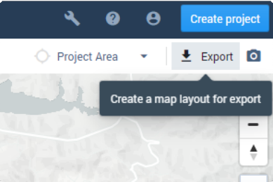
The Map Export window appears.
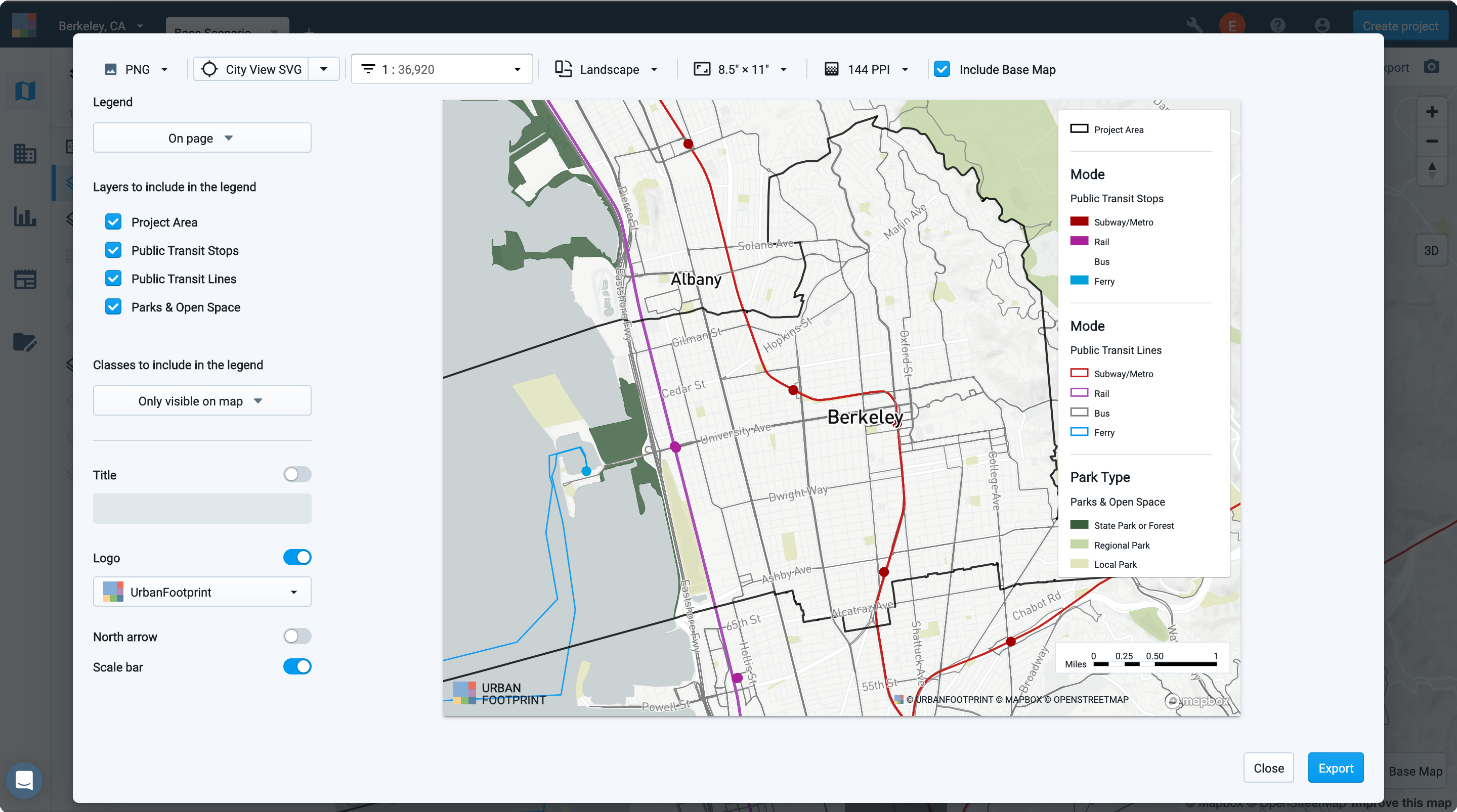
Map Export window with PNG export controls
Select the SVG export option at the top left corner of the window. Only the map export options applicable to SVG exports will remain active. All others—including controls for the map resolution, inclusion of the base map, legend, title, logo, north arrow, and scale bar—will be disabled since they are applicable only for PNG exports.
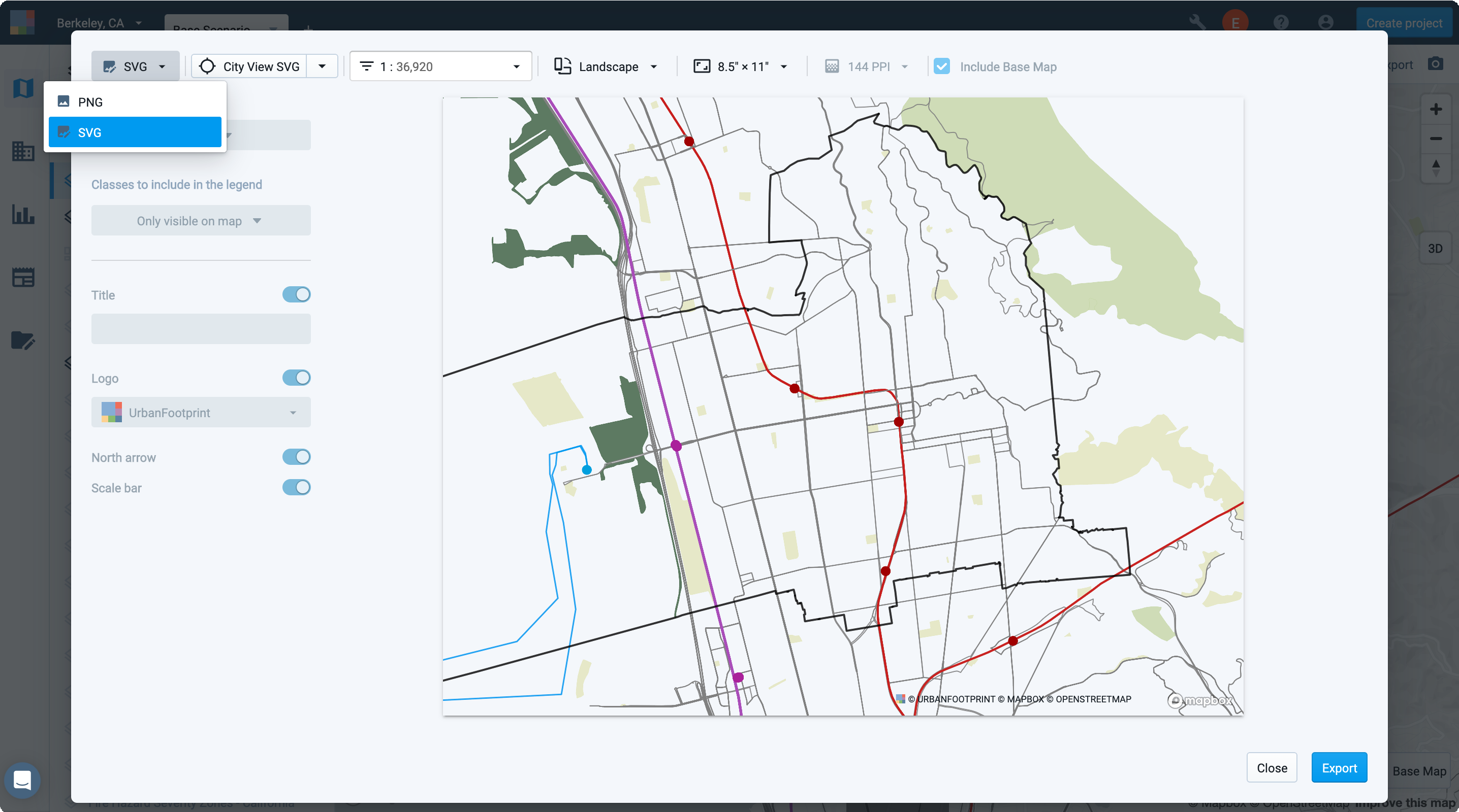
Set your map orientation and size.
Pan, zoom, and set a map scale to adjust your map view.
Save your map position. Saving your map position is recommended so you can create other maps at the same extent.
Click Export to export your map. Exporting your map will take time depending on its scope. When complete, you'll be prompted by a notification to download your map.

Note
The Export button will be disabled if your map area is too large and contains more than 300,000 features. Consider mapping a smaller area, or including fewer features or layers.
If an export is taking a very long time to complete, it's possible that the map features included are too geometrically complex. This may occur even with lower feature counts. If this occurs, please contact Analyst support for help.
Note
The file size of SVG exports increases with map size, and the number and geometric complexity of features included in the mapped layers. Large SVG files may be challenging to load and work with using Illustrator or other programs, depending on the capacity of your computer.
Click Download in the notification bar. The SVG file will be downloaded to your computer.
Open your SVG file in a vector graphics editing program. For our example, we'll look at the contents of the SVG file in Illustrator. If you use Illustrator, follow along and open the SVG map file that you exported.
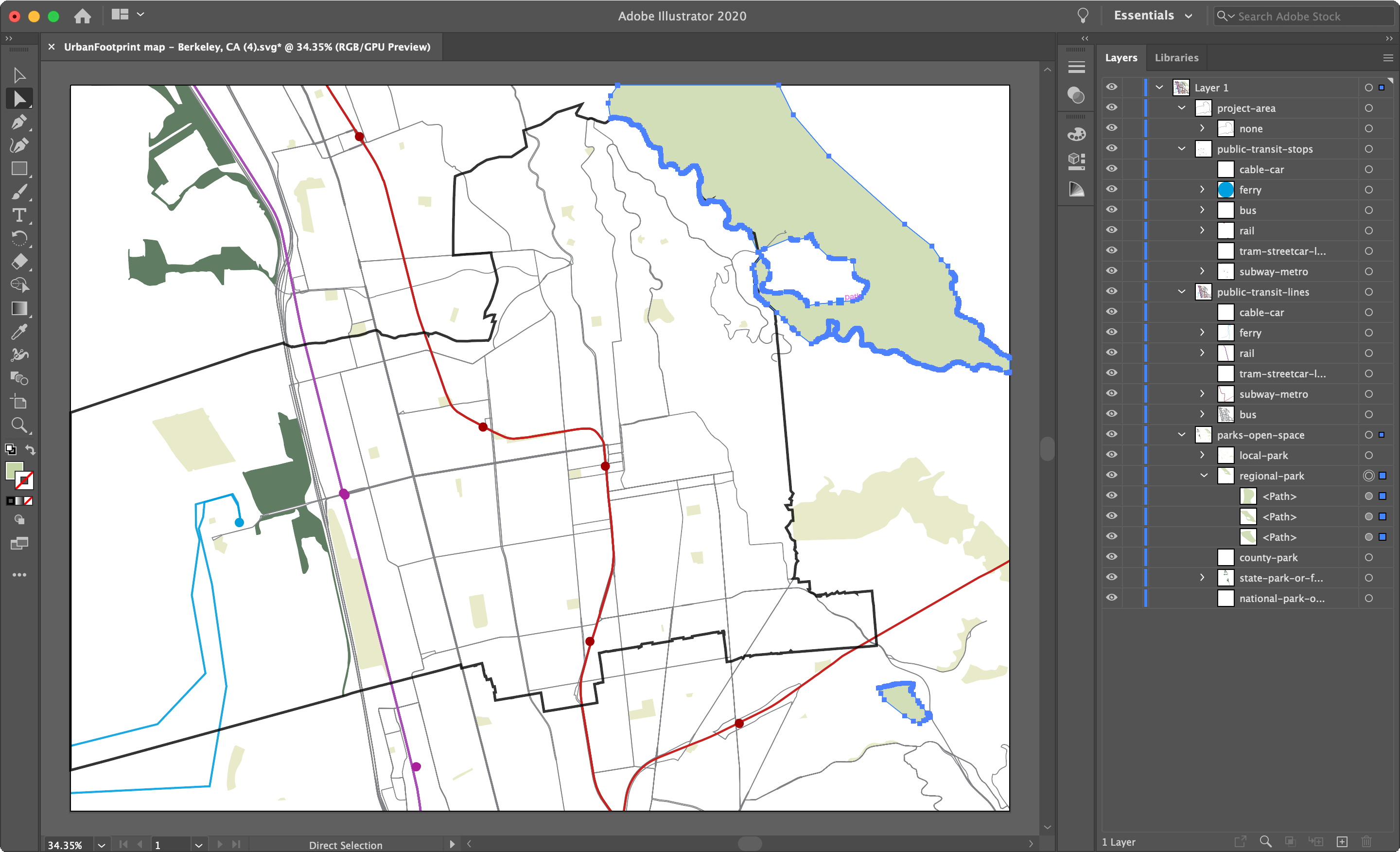
SVG file contents, shown in Illustrator
Take note of a few elements:
Grouping by layer and class – Each feature from the mapped Analyst layers is represented by a vector object. The Illustrator Layers panel shows the vector objects grouped first by Analyst data layer, then by class for the currently mapped column. For the Parks and Open Space layer in the example above, you can see that objects are grouped by park type. Here, we've selected all the "Regional Park" objects.
Style properties – All objects are symbolized using the colors and strokes as specified in Analyst.
Map extent –The area included in the SVG file matches that depicted in the Map Export view. Features that extend beyond the map area are cropped by the map edges.
Also note that SVG exports include data layers only. To export a base map image to use as an underlay, continue with the next steps.
In Analyst, hide all layers. Our plan is to export the base map on its own.
Change your base map selection, if needed. Click the Base Map control in the lower right corner of the map view. The Base Map Selection window appears. Select a base map option and features, then click outside the window to close it. (Note that if you include labels, they can get overlapped by features in your SVG file. Omit labels from the base map if you want to create custom labels in your graphics editing program.)
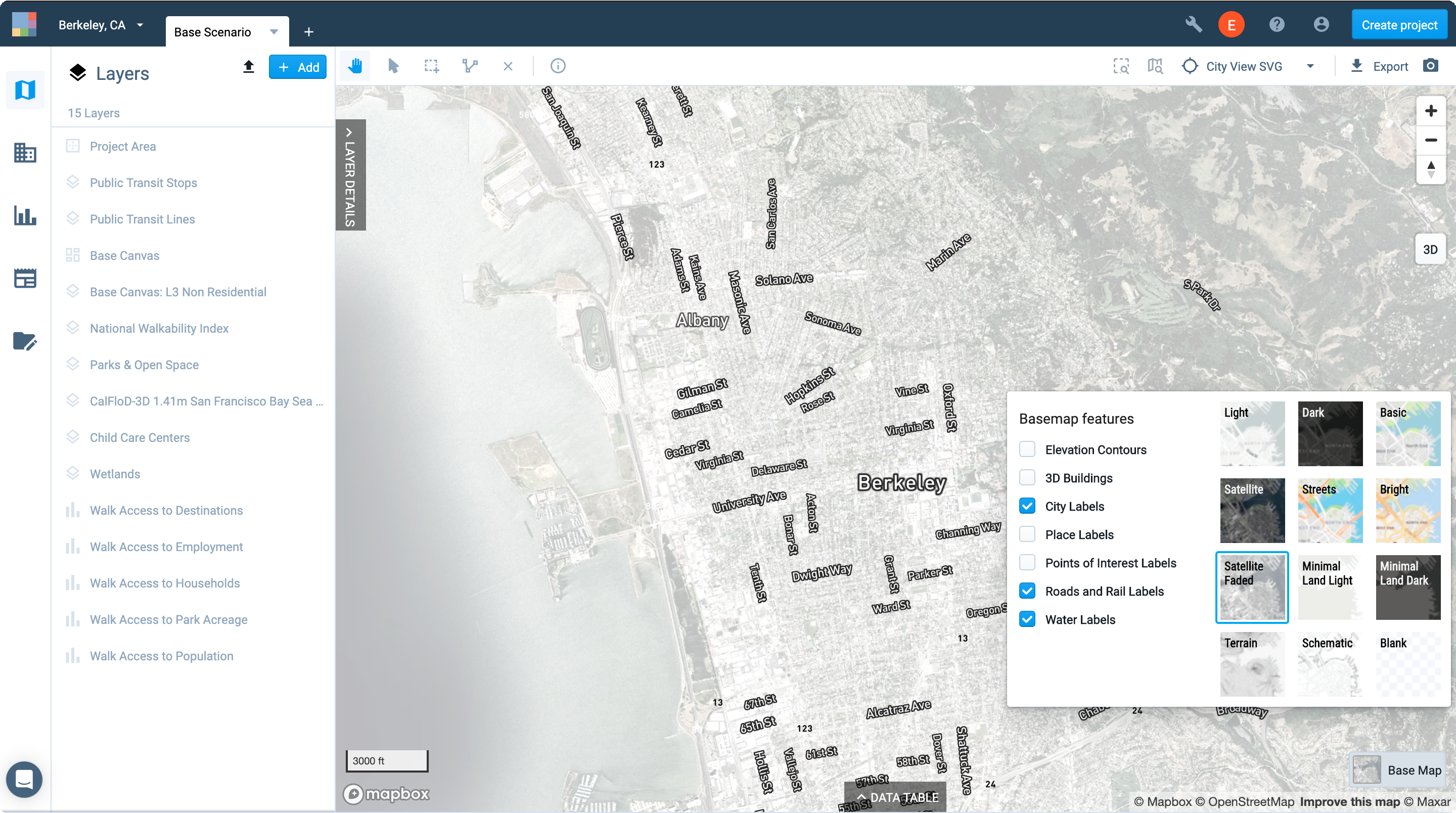
Base Map Selection window
Click the
Export button that appears above the top right corner of the map. The Map Export window appears again, this time with only the base map showing.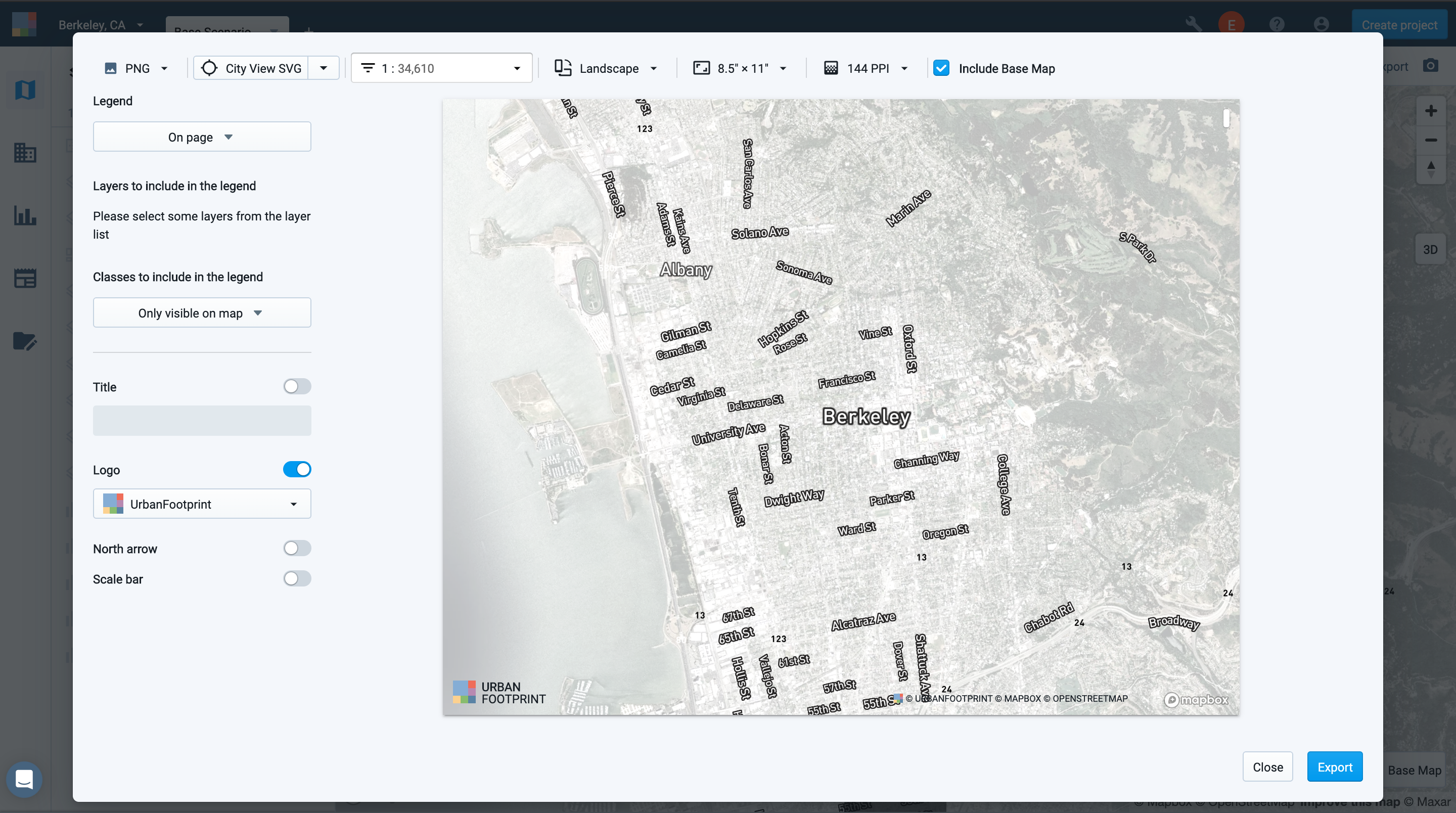
Exporting the base map
Select the PNG export option at the top left corner of the window.
Restore your saved map position. The map extent should match that of your SVG export.
Select the elements you want to include in your map. You can include a logo, north arrow, and scale bar. Keep in mind, though, that this layer will be used as a background to the vector layers in your SVG file.
Click Export to export the base map. When complete, you will be prompted by a notification to download your map.
Click Download in the notification bar. The PNG file will be downloaded to your computer.
Place the PNG file on a new layer in your SVG file. You will need to scale the PNG image to align with the edges of the SVG layer. Order the layer containing the PNG file so it sits below your feature layers. You can see our sample Illustrator file below.
SVG file with an added base map layer
Export your map to PDF format. When you have finished styling your map, you can export it to your specifications as a PDF file using the export controls of your graphics program.
Summarize Data for Subareas
While summarized scenario statistics and analysis module results are reported project-wide, you can extract results for smaller areas, or "subareas" of your project, by selecting features from your scenario canvas and analysis output layers. In this tutorial, we'll use filters to create a selection, save it as a filtered layer, and export to summarize results.
Filtered selections based on spatial criteria can be created using reference data layers (for example, to select areas within a distance of transit stations), or with the aid of dedicated layers that delineate custom boundaries (for example, a specific plan area boundary). If you're using a custom boundary, upload it to your project before starting. (See Upload Data Layers for details.)
Data Layers |
|
Features |
Upload a custom layer or create a saved filtered layer that represents your subarea boundary. For our example, we'll create a saved filtered layer for a single transit station area using the Public Transit Stops reference data layer. (While you can always select features in a subarea using on-the-fly filters, creating a subarea boundary layer in advance makes it easy to repeat subarea selections.)
From the Filter tab of the Layer Details pane for the Public Transit Stops layer, click the Add filter + button and select Mode from the list. Select Subway/Metro from the list of values that appears.
Manually select a single stop. Use the Point selection tool
 to select one stop from the filtered selection. For our example, we'll select the Ashby BART station.
Add a buffer to the selection. We're interested in a half-mile area around the station. Navigate to the Buffer tab in the Layer Details pane and enter a distance of 0.5 miles.
Click Save as to save the selection as a new buffered layer. We'll call ours Ashby BART Subarea. The new layer will appear in the Layers list.
Select the layer to be summarized. For our example, we'll summarize the scenario canvas. Click on the tab for the desired scenario, then click on the Scenario Canvas in the Layers list.
Create a subarea selection from your scenario or analysis output layer. We'll select the subarea features using a join filter. You can use a custom boundary layer, if you have uploaded one, or a saved boundary layer. We'll use the subarea boundary layer that we created for the Ashby BART station area in Step 1.
From the Filter tab, click Join and select the Ashby BART Subarea layer.
Click Save as to save the selection of features in the subarea as a new filtered layer. By saving the selection of features as a layer, you can easily return to it, or export to CSV and other formats. You can also show the subarea layer separately in maps. We'll call the new subarea layer "Scenario Canvas: Ashby BART Subarea".
Since we're working with a scenario canvas, the saved subarea layer will be dynamic. If you make changes to the scenario canvas, the content of the subarea layer will be updated to match. This is useful for summarizing data as you iterate on scenarios.
Note
While filtered layers created from the Base Canvas or scenario canvases are dynamic layers, filtered layers created from any other type of layer, including analysis outputs, are static. If analysis outputs are updated, you'll need to create a new subarea selection to summarize results.
Use the subarea layer to view data. Now we can work with the new subarea layer, which includes the scenario canvas features within the subarea.
Expand the data table. You'll see that the row count at the top right of the data table pane indicates the number of features in the subarea.
View the column summaries. With the Column Summary: Sum option selected, you can see scenario attribute totals at the top of each column. This may provide all the information you need, or you might opt to export the data for use outside Analyst.
Export the subarea data. You can export CSV data from the data table, or to other formats using layer export.
To export the CSV data, click the Export as CSV button above the data table for the subarea layer. When your export is ready, click the notification to download to your computer.
To export the subarea layer to CSV, CSV with geometries, GeoJSON, GeoPackage, shapefile, or SVG formats, use the Layer Export control at the top right of the Layer Details pane. See Export Layer Data for more details.
Summarize the CSV data. You can work with CSV data in Excel, Google Sheets, or other spreadsheet programs. Pivot tables are useful for summarizing base or scenario canvas data, as shown in the example below.
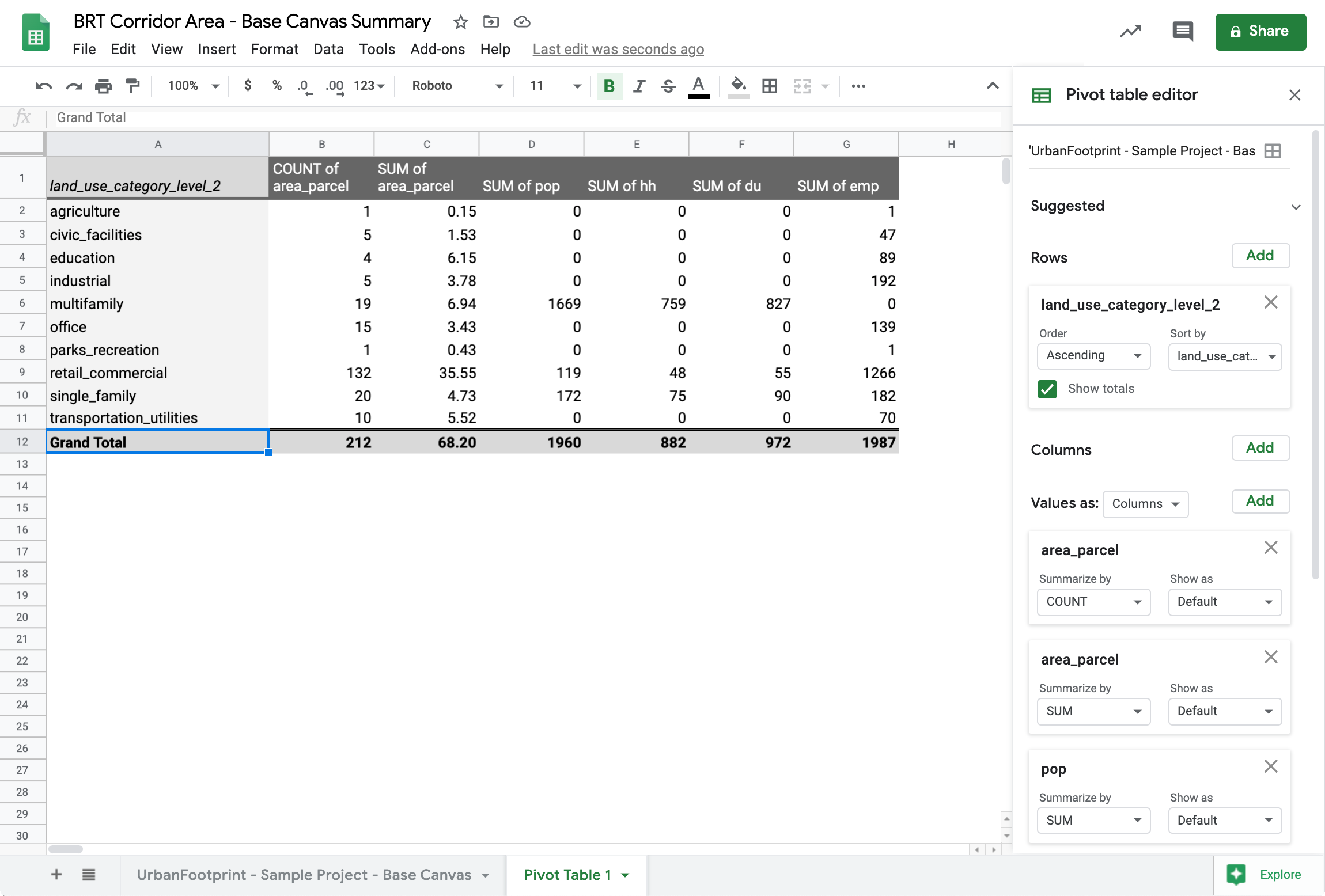
View of a Google Sheets pivot table summarizing CSV data for a subarea of the Base Canvas
Please refer to Excel help, Google help, or other resources for guidance on using pivot tables.