Transportation Analysis
The Analyst Transportation module is a high-level travel model that produces estimates of the following metrics for land use and transportation scenarios:
Vehicle miles traveled (VMT)
Trips taken, organized by mode
Transportation costs
Greenhouse gas (GHG) emissions and pollutant emissions
The Analyst Transportation module estimates VMT and mode share with sensitivities to the effects of the built environment on travel behaviors. These effects are quantified within the Analyst Transportation module according to the Mixed-Use Development (MXD) method, which consists of statistical models based on research of observed relationships between characteristics known as “D” factors and travel behavior in cities and regions across the U.S.
In turn, VMT estimates are used to calculate greenhouse gas (GHG) emissions, criteria pollutant emissions, and household auto costs. See Emissions Analysis and Household Costs for further information.
Transportation analysis is run at the resolution of the project canvas (parcels or census blocks), yielding a spatial output layer and corresponding data table; both can be used within Analyst for mapping and data exploration, and exported. The module also reports individual and comparative scenario results via summary charts, and generates a spreadsheet summary in Excel format.
Methodology
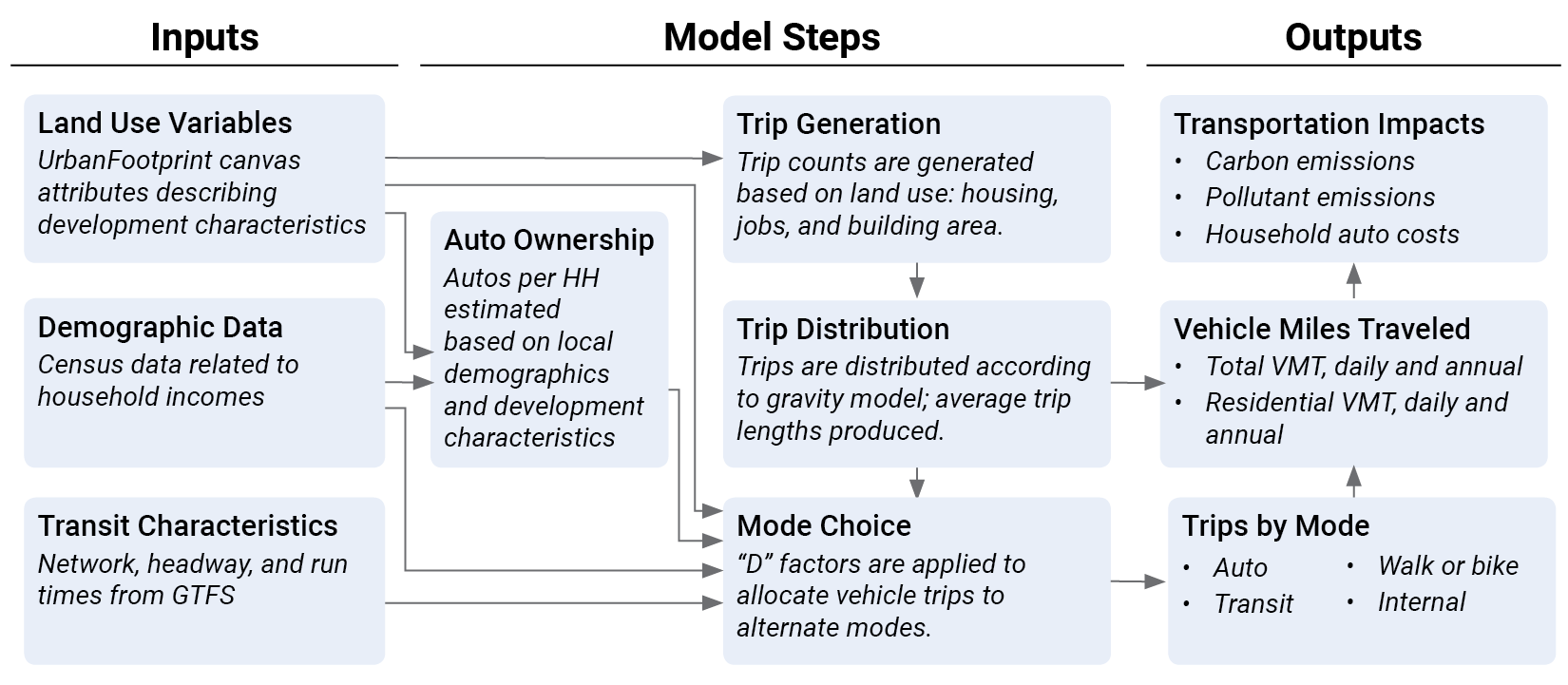
The travel forecasting capabilities of Analyst are based on a comprehensive body of research on the observed relationships between trip generation and characteristics of the built environment25. Transportation Analysis Flow summarizes the analysis flow from inputs to outputs.
 |
The Ds
Among the findings of this research is that urban form, transportation supply, and management policies affect VMT, automobile travel, and transit in at least 8 different ways. These mechanisms are referred to as the “8 Ds.”
The “8 Ds” include:
Density – residential and employment concentrations;
Diversity – jobs/housing, jobs mix, retail/housing;
Design – connectivity, walkability of local streets, and non-motorized circulation;
Destination – accessibility to regional activities;
Distance to Transit – proximity to high quality rail or bus service;
Development Scale – critical mass and magnitude of compatible uses;
Demographics – household size, income level, and auto ownership;
Demand Management – pricing and travel disincentives.
The relationships involving the first seven Ds are quantified within a segment of the core of Analyst's Transportation Module. This segment, named the Mixed-Use Trip Generation Model26 (MXD), runs the measured attributes through a series of statistical models that are based on research27 prepared for the United States Environmental Protection Agency and the American Society of Civil Engineers. The method for measuring effects of the “8D” travel engine, i.e., various demand management strategies, has been developed, but it has not been implemented in the current Analyst Transportation Module.
The study developed hierarchical models that capture the relationships between the identified “D” factors and the amount of travel generated by over 230 mixed-use developments in a wide variety of settings and sizes across the United States, including developments in the Sacramento and San Diego regions. The predictive accuracy of the methods was validated via traffic field surveys at almost 30 other development sites.
The use of “D” factors from the MXD model allows Analyst's Transportation Module to assess the comparative transportation impacts of scenario modifications to public transportation networks, urban land use, and contextual regional development patterns. With the MXD component of the Transportation Module, users are able to measure a range of factors, including:
The effects of transit development.
The impact of various densities and use mixes.
The impact of future employment location decisions.
Model Overview
The core of the current Transportation Module, the MXD method, is based on a traditional four-step travel demand forecasting model. It has three key components28:
Trip generation
Trip distribution
Mode choice modeling
Trip generation involves estimating the total number of trips associated with each of the different land uses in the project area with the standard ITE trip generation rates29. During trip distribution, these trips are allocated to likely origins or destinations. The allocation is determined via a gravity model (a description of the gravity model is provided in the Trip Distribution section overview).
Mode choice is then determined. In this step, trips are assigned a mode according to a series of observed proportional allocation rates that are determined via the previously outlined “D” categories. Specifically, this step involves estimating via a series of statistical models the degree to which an area’s external traffic generation30 will be reduced due to:
Walking or biking
Transit use for off-site travel
Trip internalization (a product of mixed use conditions, allowing a trip to remain “captured” within the site itself)31
This step enables estimation of the following:
VMT per household (daily, annual)
VMT per capita (daily, annual)
Trips by mode
In addition, this step provides the base inputs that allow for GHG emissions and household costs. The following sections describe the default assumptions and calculations of each component.
Model Assumptions
While the typical assumptions that hold true for a traditional four-step travel demand forecasting model apply to the Analyst Transportation Module, the MXD component of the module requires some additional assumptions to be set. These assumptions are used to post-process auto trips and adjust the auto mode trip counts generated from the traditional mode choice model. Broadly, the MXD model performs the following steps:
It estimates vehicle trips during the trip generation step.
It then adjusts the number of vehicle trips to reflect the impacts of “D” variables. “D” variables are factors that contribute to the reduction of the number of vehicle trips. This is explored in more detail in the trip distribution step.
There are other assumptions underlying each step of the model, which are explained in the following sections.
Trip Generation
The trip generation step applies standard ITE manual trip generation rates and generates trips associated with land uses for the project area's Base and Scenario canvas features. The method categorizes each trip as one of the following:
Home-based work (HBW) (production, attraction)
Home-based other (HBO) (production, attraction)
Non-home-based (NHB) (production, attraction)
For HBW and HBO trips, the method involves estimation of the number of external trips, which are trips that originate or end in areas external to the Analyst project area.
Calculations
To estimate the number of vehicle trips either produced or attracted to a given parcel, the standard ITE trip generation rates are used to generate initial vehicle trip counts. These rates differ according to the target parcel's household type and employment sector composition. They are discussed in more detail in the Input Parameters section (regarding the default rates used in the system).
For trips associated with residential land uses, trip generation accounts for three residential dwelling unit types:
Single-family dwellings
Multifamily dwelling with 2-4 units
Multifamily dwelling with 5 or more
In the trip generation step, the number of trips produced by households is estimated by multiplying the number of occupied residential dwelling units of a given type by the corresponding stated trip generation rate. For example, the number of trips produced by households living in single-family dwelling units is given by the following equation:
The logic for estimating trips associated with other land uses is similar. In the trip generation step, the number of trips associated with the following eight non-residential land uses are calculated:
Retail
Restaurant
Entertainment
Office
Public
Industry
School (K-12)
School (College/University)
For typical employment, trips are calculated according to the following equation:
Trips associated with retail, entertainment, and restaurant destinations are handled differently than other trips are handled. Their numbers are calculated via the following equation (explained in detail after the equation):
For these particular trips (retail, entertainment, and restaurant), an alternate estimate of the number of jobs is used. This estimate is determined according to set area-job conversion rates that describe the average number of jobs per building area for various programming types. The default rate is two jobs for every 1,000 square feet of building area.
Total K-12 school trips are estimated as a percentage of total residential trips. The module uses a default rate of 0.097 (K–12 school trip per residential trip)32. Currently the number of college/university trips defaults to zero in the released version of the module in Analyst.
Trips are re-grouped into the following five categories:
Retail (includes retail, restaurant, and entertainment)
Office (including office and public)
Industrial
School (K–12 and higher education)
Residential (including single-family and multifamily dwelling units)
These trips are further grouped by subcategory and direction (attraction or production). Currently the module considers three trip subcategories:
Home-based work (HBW)
Home-based other (HBO)
Non-home-based (NHB)
The National Cooperative Highway Research Program (NCHRP) person trip rates33 have been adapted for identification of the proportion of total trips that are allocated to each trip category. These proportions are used to weight the previously computed trip counts (which are based on ITE trip generation rates) into the trip categories. For a better understanding of the application of the NCHRP person trip rates, an example focusing on residential trips is set out below.
First, assume there are Nr occupied residential dwelling units (DU) for a given parcel. Current default rates for the module are as follows:
Production trips
8.85 daily person trips are generated per residential dwelling unit34. The default distribution of production trips is as follows.
21% are home-based work (HBW)
56% are home-based other (HBO)
23% are non-home-based (NHB)
Attraction trips
No HBW attraction person trips are produced.35
0.9 daily HBO person trips per residential dwelling unit are generated.
0.5 daily NHB person trips per residential dwelling unit are generated.
These factors are represented in N, is the number of residential dwelling units per parcel.. In this table, each category represents a percentage of the total trips. The calculation in each cell illustrates the previously generated ITE residential trips.
Trip Type | Production Trips | Attraction Trips |
|---|---|---|
Home-based work (HBW) | Nr * 8.85 * 21% | Nr * 0 |
Home-based other (HBO) | Nr * 8.85 * 56% | Nr * 0.9 |
Non-home-based (NHB) | Nr * 8.85 * 23% | Nr * 0.5 |
In the Analyst Transportation module, all residential NHB production trips36 are, by default, external trips with both trip ends outside the project area. Specifically, it is assumed that:
0% of residential NHB production trips are internal-external trips, and
0% of residential NHB production trips are external-internal trips.
To accommodate this assumption, all residential production trips that are NHB are removed. Next, HBW and HBO other trips are scaled up proportionally to replace the removed NHB trip counts. In other words, residential NHB production trips and associated VMT are attributed to residents in the project area no matter if they are external or internal to the project area.
The same process is used for other non-residential trips. In each instance, proportions are calculated according to the paired NCHRP data for each trip type.
The last step of trip generation is categorizing the trips in each category as internal or external. By definition, both ends of internal trips lie within the project area. On the other hand, external trips either originate or end in areas outside of the project area.
Currently, the module only estimates external HBW trips, primarily because of the limited availability of datasets for building estimation models (to predict external percentages for HBO and NHB trips).
A percentage of HBW trips will be designated external trips, allowing for the balance of internal-internal production and attraction trips in the project area. For each project, the percentage of trips types where either the origin or the destination is external to the project site is estimated via a Decision Tree (DT). A DT is a non-parametric supervised learning method that we employ to develop a regression within the model.
The decision tree algorithm first finds similar projects, in a pool of representative project samples, as the target project. It does so by categorizing all projects based on a list of attributes, such as employment household ration, sum of dwelling units by type, and summary stats of intersection density37. The algorithm then predicts the external trip percentage for the target project by taking a weighted average of external trip percentages of those similar projects.
The final output of trip generation is vehicle trip counts categorized according to whether they are internal or external, whether their purpose is HBW, HBO, or NHB, and whether they are production or attraction trips.
Trip Generation Input Parameters
Average trip generation rates by category presents default trip generation rates used to estimate the number of residential and non- residential trips in each category. 383940
Single Family Detached | 9.57 vehicle trips per household |
|---|---|
Single Family Attached | 6.65 vehicle trips per household |
Multifamily | 4.18 vehicle trips per household |
Retail | 42.94 vehicle trips per thousand square feet |
Restaurant | 75 vehicle trips per thousand square feet |
Entertainment | 20 vehicle trips per thousand square feet |
Office | 3.32 vehicle trips per job |
Public | 3.32 vehicle trips per job |
Industry | 3.02 vehicle trips per job |
Trip Distribution
While the trip generation step determines the number of trips that will occur in a given parcel or block, it does not specify the destination or origin of trips. The specification of trip destinations occurs during the trip distribution step.
The Analyst Transportation Module applies a gravity model to pair trip origins with destinations. This is the most common trip distribution method used in four-step travel demand forecasting models. The key assumption behind the gravity model is that people are more likely to travel to areas that feature more “attraction” and less “travel cost.” There are alternative methods of generating trip aggregations for distributing trips in a travel demand forecast process, such as the growth factor method41 and the disaggregate trip distribution method42.
Destination “attraction” and “travel cost” can be calculated in several ways. Based on a gravity model, the following equation43 provides an overview of the logic behind the trip distribution method as it is used in the Transportation Module.
Variable definitions (TAZ is an abbreviation for “traffic analysis zone”):
Tp is the number of trips of type p, from TAZ i to TAZ j.
Pp is the number of trip origins of type p in TAZ i, generated during the trip generation step.
Ap is the number of trip destinations of type p in TAZ j, which is generated during the trip generation step.
f(t )is a function that outputs the cost of traveling between TAZ i and j; it is usually a function of travel time.
K represents adjustment factors for travel flow between TAZ i and j; they account for the possibility that factors not captured in the rest of the model influence destination choices.
In essence, this step allocates trips to traffic analysis zones (TAZs) according to two factors: zonal attraction strength and travel expenses. The following section provides more details about how these variables are calculated and the default parameters and equations used in the trip distribution step.
Calculations
Internal and external trips are distributed slightly differently. For internal trip distribution, all calculations are performed at the traffic analysis zones scale, which is a commonly used geography for travel demand forecasting. All evaluated blocks or parcels will be paired with their parent TAZ, and they will have descriptive attributes inherited from their parent TAZ.
During the trip generation step, trip origins and destinations are determined for each Canvas Geometry based on Land Use Types, Employment Densities, and other resources. These results are aggregated from the Canvas Geometries to the Census TAZs that they lie within and inform the full distance matrix of that scenario.
Next, a full distance matrix is computed. That is, the cost of travel between any two pairs of TAZs is calculated. Travel cost can be measured in various ways. It can be as simple as travel distance or as complex as a composite measure that includes various kinds of travel times (e.g., traffic data) and costs.44
By default, the module calculates a modified city grid distance between TAZ centroids and uses it as travel cost. City grid distance is based on the assumption that the relationship between an isosceles triangle’s hypotenuse and two other sides (adjacent and opposite) is roughly modeled by the average circuity of an “as the crow flies” direct line distance and the real path necessitated by the urban road network. Thus, to calculate the “real” distance between two centroids, one would multiply the straight point-to-point distance by the square root of 2 (approximately 1.4142). This value has been increased slightly because of a nationwide study of driving distance versus straight line distance to the nearest hospitals. That is, what was the distance more than the direct, straight line distance that a vehicle had to travel to reach its destination by traveling on available road networks. The study found an average percent difference (that is, a circuity factor) of 1.417.45 This circuity factor will be available to users and adjustable for site optimization.
The output of this step is a matrix with the following composition:
Rows represent the cost of a trip originating from one TAZ to all others
Columns represent the cost of a trip from each of the other TAZs to one TAZ
Costs are calculated via the (aforementioned) modified city-grid distance between an origin TAZ and a destination TAZ. Trips internal to TAZs are assigned an “average trip length.” This value is calculated by measuring the radius of the smallest circle encompassing the largest single geometry of a given TAZ’s composite geometries (polygons).
The travel distance matrix is then transformed into a travel impedance matrix via a deterrence function, a common method for representing the nonlinear impacts of travel cost changes on travel choices. The module uses an exponential deterrence function and a default initial β of 5. See Input Parameters for more details.
The next step is generating an initial trip matrix, assuming the K factors are equal to 1.46 During this step, TAZ i, for example, is taken, which has a number of home-based work trip origins equal to Pi. Pi is allocated to all the TAZs (including itself) according to the equation:
Note that the summation of the above for TAZ j should be equal to 1. In other words, more trips are allocated to TAZ j if it has more trip ends, indicating that it has a larger population and/or more employment (and therefore more “attraction”) if it costs less to travel to, which in this case means being closer to TAZ i.
Depending on the scale of travel impedance values and initial deterrence function parameters, the resulting matrix may contain invalid values as a result of extremely small denominators. To account for this, the module automatically adjusts deterrence function parameters according to a simple decay function. Users can set minimum deterrence function parameters. Currently, the module’s minimum β value for the exponential deterrence function is 0.01.
The next step is balancing the matrix via an iterative proportional fitting (IPF) technique47. The initial trip matrix generated during the previous step is an unbalanced matrix because the sum of the allocated trips for each destination TAZ (that is, the sum of the values in each column) does not necessarily match the number of attraction trips estimated during the trip generation step.
Thus, the primary purpose of this step is to adjust trips proportionally until the resulting trip matrix matches the trip generation estimates. Therefore, at this stage the module calculates:
The ratios of the sum of the trips allocated for destination TAZs to the estimated number of attraction trips for destination TAZs, and
Scaled counts of trips that end in a given TAZ (using the corresponding ratio).
The consequence of this operation is that the number of trips allocated for each origin TAZ is not necessarily equal to the number of production trips estimated for each TAZ. That is, during the first pass, trip allocation does not necessarily match the pre-assessed production trip count for a given TAZ. As a result, each successive iteration scales up the production trips for each TAZ by each TAZ’s corresponding ratio (that is, its ratio of allocated trips to the previously computed production trip count “source of truth”). It is this balancing operation that is “iterated” until convergence. For more information on the application of IPF to trip distribution, please refer to chapter 5 of “Modeling Transport” (Ortuzar, Juan de Dios and Willumsen, Luis G.).
In this model, the iterative balancing repeats until one of the following thresholds is met, the first two of which have parameters the user can control:
The sum of the trip origins and destinations for each TAZ differs from the values estimated during the trip generation step (the degree to which this is allowed to be off is customizable by value from 0 to 1).
A maximum of 5,000 iterations has been reached.
The iteration step has run for longer than 5 minutes without successfully converging (that is, satisfying either threshold 1 or 2).
A simplified version of the method above is applied when assigning trips to areas that lie outside the project area. Because a 150-kilometer buffer area is used to identify development in a broader area in around the project site, the number of Canvas Geometries being evaluated may increase by several orders of magnitude. (Note that this buffer area does not correspond to the optionally defined context area for a project, or the "access area" used by the Walk and Transit Accessibility modules.)
The above approach to distributing external trips would require processing all geometries in the outlying buffer area. To reduce the computational expense, the buffer area is preprocessed to reduce the number of possible origins and destinations external to the project area to a limited series of representative points.
To create the buffer area’s summary point, the module searches for likely origins and destinations according to employment and household densities in the buffer area48. Using these attributes, a kernel density estimation (KDE) algorithm smooths data to generate discrete peaks in the project’s surrounding buffer area. Among these peaks, a limited set of external locations are identified, and all external trips starting or ending in the project area will be distributed (to or from) these locations.
External trips are distributed to potential locations according to:
The distance between two locations.
The further a location is from the origin, the less likely a trip will be taken.
How attractive or generative the external location is.
Attraction is measured in terms of employment densities.
Generation is measured in terms of household densities.
The last step of the trip distribution component of the Transportation Module is calculating an average trip length for each trip category. Below is a walkthrough of this step with examples of home-based work production trips.
In this step, the weights are equal to the quotient of the number of trips from TAZ i to a given destination and the counts of the trip origins of TAZ i. The average production trip lengths from TAZ i are calculated next. These are equal to the product of the distances between each TAZ i and the other TAZs, and the corresponding weights, as shown in the following equation:
Variable definitions:
AverageTripLength ⁿ represents the average home-based work production trip length for location i.
Distance is the distance between locations i and j (the Origin Centroid-to-Destination Centroid within the Traffic Analysis Zone distance by default).
N is the number of home-based work trips from location i to j.
P is the number of home-based work trip origins produced by location i
(Note that this count value comes from the trip generation step.)
Trip Distribution Input Parameters
Forms of Deterrence Functions presents the deterrence functions available to users. Users can also adjust the coefficient parameters used in each deterrence function available.
Deterrence Functions | Forms | Parameters | Default Values |
|---|---|---|---|
exponential function | Equation 20. | β | 5 |
power function | Equation 21. | n | - |
combined function | Equation 22. | β, n | - |
gamma function | Equation 23. | a, b, β | - |
In the formulas above, c is the raw cost of traveling between origin i and destination j. What it represents can be as simple as travel distance or as complex as a generalized cost that includes various other factors.
Mode Choice Modeling
The core of the MXD method is a series of logistic regression models, which are used to estimate the degree to which the traffic generation of a given development area will be reduced because of a variety of contextual factors, including:
Development density
Diversity
Design
Destination accessibility
Distance to transit
Demographics
Development scale
These attributes (known as “D” factors) are all associated with the likelihood of walking, transit, or internalized trips associated with each parcel.
This method enables the model to be sensitive to differences amongst a broad array of land use types, which are used to depict development in scenarios. This sensitivity is achieved via calculation of the vehicle trip reductions resulting from the combination of “D” variables that are based on their land use characteristics.
“D” characteristics for each canvas feature are measured based on the characteristics of the feature itself, along with the characteristics of neighboring features within a buffered distance. The buffered distances differ for each variable, as indicated in Explanatory and outcome variables in MXD equations (see "Explanatory Variables").
Mode Choice Calculations
A logistic regression model predicts the probability of an event according to the variable attributes assigned to each geometry in the broader area. In this context, the model is used to determine whether a trip is a vehicle trip or a walk, transit, or internal trip. This determination is based on a series of variables and the following equation:
The variable t is a linear function of one or more variables and is referred to as “log-odds”49 and is described by the following equation:
The operator Ln indicates the natural logarithm of each built environment “D” variable (VAR in the equation above). The result of this operation is multiplied by a variable-specific coefficient (Coeff in the equation above).
The results of the calculation for each variable VAR are summed and added to the variable Constant, which produces the logarithmic odds of travel being an internalized, pedestrian, or transit trip. The variables of the MXD equations are listed below.
Variable | Explanation |
|---|---|
Outcome Variables | |
Internal | Trip remains within the parcel (1=internal, 0=external) |
Walk | Travel mode of an external trip is walking (1=walk mode, 0=other) |
Transit | Travel mode of an external trip is bus or rail (1=transit, 0=other) |
Explanatory Variables | |
AREA | Gross land area within the parcel. |
EMP | Employment within the parcel. |
ACTDEN | Resident population plus employment per square mile of gross land over a quarter-mile buffer of the parcel. |
JOBPOP | Average jobs/housing balance (index comparing the local ratio to the “ideal” regional average) over a quarter-mile buffer of the parcel. |
INTDEN | Number of intersections per square mile of gross land within or within 400 meters of the parcel. |
EMPMILE | Total employment within 1 mile of the parcel. |
EMP30T | Total employment within a 30-minute transit trip from the parcel. |
Explanatory and outcome variables in MXD equations contains two sections, “Outcome Variables” and “Explanatory Variables.” The second section, “Explanatory Variables,” is often associated with the “D” variables that affect trip generation. These include development density, diversity, design, destination accessibility, distance from transit, development scale, and demographics. The output of the hierarchical modeling involved in the MXD model’s research and development included the individual and combined effects of the seven types of “D” variables on the travel characteristics of 239 targeted mixed-use development areas. Via this research, the variables above were determined significant.
Analyst dynamically calculates these explanatory variables at the appropriate resolution using the current scenario’s canvas data. In other words, these variables reflect different land use patterns and other built environment characteristics of each scenario that a user creates. To ensure that explanatory variables reflect “average” characteristics of a given parcel and its surrounding, various sizes of buffers are applied to derive representative measures of each location. For example, a quarter-mile buffer is used to derive resident population and employment density that is representative of local activity level of a given parcel.
However, such calculation can be computationally intensive, depending on its implementation, especially for large projects that contain hundreds of thousands of canvas shapes. To ensure that the Transportation Module can finish within a reasonable amount of time even for large parcel projects, data are aggregated to standard grids. With that, efficient algorithms can be applied, which allows quick generation of explanatory variables for all canvas shapes in a project.
For internal capture, the dependent variable is the natural log of the odds of an individual making a trip whose origin and destination lie within the same parcel. Depending on the trip-purpose, this probability is related to the development scale, a variety of mixed-use land variables, the measured urban design quality of the MXD, and several demographic variables. The log-odds probability of walking to external destinations is related to the MXD’s size, density, development mix, urban design, demographics, and the number of jobs within a mile. The probability of a vehicle trip being shifted to a transit trips is a function of demographics and the accessibility of the site’s transit to the rest of the region. This accessibility is expressed in terms of jobs within a 30-minute transit trip. The tables in the “Input Parameters” section present the values of parameters used in the log-odds equation.
Mode Choice Input Parameters
The following tables present the relationships used in the following equation:
The constant term, variables (VAR), and coefficients (Coeff) are presented in Log-odds of internal capture (log-log form), Long-odds of walking trips (log-log form), Log-odds of transit trips (log-log form).
Variable | HBW | HBO | NHB | ||||||
|---|---|---|---|---|---|---|---|---|---|
Coeff | t-stats | p-value | Coeff | t-stats | p-value | Coeff | t-stats | p-value | |
Constant | -1.75 | -2.43 | -5.32 | ||||||
EMP | - | - | - | - | - | - | 0.208 | 3.28 | 0.002 |
AREA | - | - | - | 0.486 | 3.61 | 0.001 | 0.468 | 4.58 | <0.001 |
JOBPOP | 0.389 | 2.62 | 0.01 | 0.399 | 4.55 | <0.001 | - | - | |
INTDEN | - | - | - | 0.385 | 1.92 | 0.055 | 0.638 | 4.95 | <0,001 |
HHSIZE | -1.33 | -6.03 | <0.001 | -0.867 | -13.0 | <0.001 | -0.237 | -4.54 | <0,001 |
VEHCAP | -0.990 | -4.15 | <0.001 | -0.59 | -8.19 | <0.001 | -0.163 | -3.0 | 0.003 |
Variable | HBW | HBO | NHB | ||||||
|---|---|---|---|---|---|---|---|---|---|
Coeff | t-stats | p-value | Coeff | t-stats | p-value | Coeff | t-stats | p-value | |
Constant | -5.55 | -10.96 | -15.09 | ||||||
AREA | - | - | - | -0.415 | -4.27 | <0.001 | - | - | |
ACTDEN | - | - | - | 0.37 | 2.74 | 0.007 | 0.377 | 3.12 | 0.003 |
JOBPOP | 0.226 | 2.46 | 0.015 | 0.219 | 3.83 | <0.001 | - | - | |
INTDEN | - | - | - | - | - | - | 0.803 | 5.05 | <0.001 |
EMPMILE | 0.385 | 3.12 | 0.002 | 0.45 | 5.05 | <0.001 | 0.44 | 5.09 | <0.001 |
HHSIZE | -1.57 | -6.29 | <0.001 | -0.486 | -5.05 | <0.001 | -0.281 | -2.59 | 0.01 |
VEHCAP | -1.84 | -7.00 | <0.001 | -0.768 | -7.62 | <0.001 | -0.242 | -2.13 | 0.033 |
Variable | HBW | HBO | NHB | ||||||
|---|---|---|---|---|---|---|---|---|---|
Coeff | t- stats | p- value | Coeff | t- stats | p- value | Coeff | t- stats | p-value | |
Constant | -8.05 | -6.08 | -2.69 | ||||||
ACTDEN | - | - | - | 0.324 | 2.89 | 0.005 | - | - | |
INTDEN | 1.12 | 4.44 | <0.001 | - | - | - | - | - | |
EMP30T | 0.209 | 2.98 | 0.004 | - | - | - | 0.134 | 3.29 | 0.002 |
HHSIZE | -1.14 | -6.31 | <0.001 | -0.958 | -8.48 | <0.001 | - | - | |
VEHCAP | -1.68 | -8.56 | <0.001 | -1.09 | -8.91 | <0.001 | -0.34 | -3.74 | <0.001 |
The logistic regression model, shown below, transforms log-odds (t) into probabilities. This transformation is represented by the following equation:
For each trip category of all internal trips (i.e. trips with both trip ends inside the project area), the probability of each trip being internal captured, or a walking or transit trip is calculated. The probability is then used to calculate the number of non-vehicle trips (internal capture, transit, and walk) in each of the three trip categories (HBW, HBO, and NHB).
For example, let’s say that the probabilities of internal capture, walking, and transit trips for internal HBW trips in a parcel are 5%, 10%, and 15% respectively. Given that the total number of internal HBW trips is 10000, the probabilities would result in the following trip distribution:
500 internal capture trips, or 5% of all internal HBW trips
1,000 walking trips, or 10% of all internal HBW trips excluding internal capture trips
1,500 transit trips, or 15% of all internal HBW trips excluding internal capture trips
If the examined trips are external trips, we only consider the probability of it being transit trip, not walk or internal capture trip.
VMT is then calculated according to adjusted vehicle trip counts and the corresponding estimated trip lengths. Vehicle trips are first categorized as production or attraction trips according to the production and attraction trip ratio derived in the trip generation step. Take internal HBW production trip as an example. It is calculated via the following equation:
After the number of trips and the corresponding trip length have been computed, the module can calculate VMT.
The module produces a set of MXD vehicle trip variables and a set of VMT variables as the main spatial outputs. The remainder of this section of the documentation will cover how different VMT variables are derived. It will also cover how the results of these operations are summarized for project-wide outputs. These summary operations are applied both to the processed VMT outputs and MXD vehicle trip outputs in a similar fashion.
The module produces both total VMT and VMT per capita (or per household). For the estimation of VMT per capita or per household, only HBW and HBO production trips are considered because they are trips produced by individuals or households in that given parcel. The VMT associated with trips that are attributed to a retail shop in this geometry or a visitor to the area, for example, is not part of this measure.
Let’s take HBW vehicle trips as an example. HBW VMT per household at the parcel level is calculated in two steps. First, the HBW VMT is calculated via the following equation:
Note that HBW attraction vehicle trips are not included in the equation above because they are not taken by households or individuals living in the given parcel.
Second, VMT per household (or capita) is determined via the following equation:
The same logic applies to calculating the per capita and per household VMT associated with HBO vehicle trips. Since residential NHB trips are assumed to be zero in the trip generation step, there is no NHB VMT associated with households50. As a result, VMT per household is the sum of HBW VMT per household and HBO VMT per household only:
When it comes to total VMT, the calculation is slightly different. Total VMT for a given parcel includes the VMT associated with not only trips generated from the geometry but also trips attracted to the area.
Again, let us take HBW vehicle trips as an example. To get the total daily VMT associated with internal HBW vehicle trips for a given parcel, the following equation is used:
VMT associated with HBO and NHB, internal or external, are derived using the same functions. Last, total daily VMT, for each parcel, includes VMT of all trip types:
Total annual VMT is derived by applying an annual factor and users can modify this factor:
The module also estimates total daily and annual VMT for the entire project area. Note that it is not the sum of previously derived total daily/annual VMT for each parcel because some trips will be double counted in the process of simply summing all parcels’ total daily/annual VMT.
The reason for this double counting is that half of internal HBW or HBO production trips are trips from home to work/other destinations. As a result, these trips are considered internal HBW or HBO attraction trips in another geometry and will be counted as part of total VMT for that geometry as well. Similarly, one parcel's internal NHB production trip can be another parcel’s internal NHB attraction trip. Essentially, variables at each parcel capture attributes of trip ends whereas project-level variables capture attributes of trips.
The following equation is used to handle the aforementioned double counting issue:
The sum of AdjustedTotalDailyVMT of all parcels is used as the project-level total daily VMT.
Note that double counting is not an issue in the external VMT calculation because the origins/destinations of external trips are outside the project area. In addition, external HBW attraction trips and associated VMT are not typically included in total VMT because they are produced by residents living outside the project area.
The module also estimates the VMT of heavy trucks by applying a truck adjustment factor. Users can modify this factor.
Output Metrics
The Transportation module generates two mapped spatial output layers and corresponding data tables; all can be used within Analyst for mapping and data exploration, and exported. The spatial layers summarize trip counts for each mode and type, and daily and annual VMT in total, per capita, and per household.
The module also reports individual and comparative scenario results via summary charts, and generates a spreadsheet summary in Excel format. The attributes of the spatial output/data tables are summarized in the Transportation Module Outputs: Vehicle Miles Traveled Table.
Transportation Module Outputs: Vehicle Miles Traveled Table
Attribute(s) | Description |
|---|---|
Population, Dwelling Units, Households, Employment | Demographic variables as depicted in base or scenario canvas. |
Autos per Household | Number of autos per household, as estimated by the model. |
VMT Annual | Vehicle miles traveled (VMT) annually in a parcel, including all passenger vehicle VMT attributed to residents, workers, and visitors in the given area. The relationship between daily a annual VMT is dependent on the “annualization factor” parameter (a default value is 350). |
VMT Annual with Heavy Trucks | VMT Annual with the addition of VMT by heavy trucks in a parcel. VMT by heavy trucks can be estimated optionally as a factor relative to passenger VMT. |
Residential VMT Annual | Annual passenger vehicle VMT attributed to residents in a parcel. Resident VMT is lower than total VMT, and will be zero without households. |
Residential VMT Annual per Household | Average annual residential VMT per household a parcel. |
Residential VMT Annual per Capita | Average annual residential VMT per capita in a parcel. |
VMT Daily | Vehicle miles traveled (VMT) daily in a parcel, including all passenger vehicle VMT attributed to residents, workers, and visitors in the given area. |
VMT Daily with Heavy Trucks | VMT Daily with the addition of VMT by heavy trucks in a parcel. VMT by heavy trucks can be estimated optionally as a factor relative to passenger VMT. |
Residential VMT Daily | Daily passenger vehicle VMT attributed to residents in a parcel. Resident VMT is lower than total VMT, and will be zero without households. |
Residential VMT Daily per Household | Average daily residential VMT per household in a parcel. |
Residential VMT Daily per Capita | Average daily residential VMT per capita in a parcel. |
Summary Chart Outputs | |
Annual total VMT | Total annual vehicle miles traveled in the project area. |
Average Annual VMT per Capita | Average annual per capita home-based passenger vehicle miles traveled in the project area. |
Average Annual VMT per Household | Average annual home-based passenger vehicle miles per household traveled in the project area. |
Average Annual VMT per Capita by Land Development Category | Average annual home-based passenger vehicle miles per capita traveled in urban, compact, standard, and rural areas, in the project area. |
Average Annual VMT per Household by Land Development Category | Average annual home-based passenger vehicle miles per household traveled in urban, compact, standard, and rural areas, in the project area. |
Transportation Module Outputs: Vehicle Trip Counts by Type Table
Attribute(s) | Description |
|---|---|
Population, Dwelling Units, Households, Employment | Demographic variables as depicted in base or scenario canvas. |
Autos per Household | Number of autos per household, as estimated by the model. |
Internal Trips Daily | Daily “internal” trips that take place within a local mixed-use area and attributed by the MXD model to residents, workers, and visitors in the given parcel. |
Walk (or Bike) Trips Daily | Daily walk, bike or other active trips shifted away from autos, and attributed by the MXD model to residents, workers, and visitors in the given parcel. |
Transit Trips Daily | Daily transit trips attributed by the MXD model to residents, workers, and visitors in the given parcel. |
MXD Vehicle Trips Daily | Daily vehicle trips attributed by the MXD model to residents, workers, and visitors in the given parcel. |
MXD Vehicle Trips Daily per Capita | Daily vehicle trips per capita attributed by the MXD model to residents in the given parcel. |
MXD Vehicle Trips Daily per Household | Daily vehicle trips per household attributed by the MXD model to residents in the given parcel. |
MXD Home-based Work Trips | Daily home-based work vehicle trips attributed by the MXD model to residents, workers, and visitors in the given parcel. |
MXD Home-based Other Trips | Daily home-based other vehicle trips attributed by the MXD model to residents, workers, and visitors in the given parcel. |
MXD Non-home-based Trips | Daily non-home-based work vehicle trips attributed by the MXD model to residents, workers, and visitors in the given parcel. |
ITE Vehicle Trips Daily | Daily vehicle trips attributable to residents, workers, and visitors in the given parcel, as estimated by ITE vehicle trip generation rates. |
ITE Home-based Work Vehicle Trips Daily | Daily home-based work trips attributable to residents, workers, and visitors in the given parcel, as estimated by ITE vehicle trip generation rates. |
ITE Home-based Other Vehicle Trips | Daily home-based other trips attributable to residents, workers, and visitors in the given parcel, as estimated by ITE vehicle trip generation rates. |
ITE Non-home-based Vehicle Trips | Daily non-home-based trips attributable to residents, workers, and visitors in the given parcel, as estimated by ITE vehicle trip generation rates. |
Walk (or Bike) Mode Share | Walk or bike mode share of all trips attributed by the MXD model to residents, workers, and visitors in the given parcel. Walk or bike share includes all internal trips. |
Transit Mode Share | Transit mode share of all trips attributed by the MXD model to residents, workers, and visitors in the given parcel. |
Auto Mode Share | Auto mode share of all trips attributed by the MXD model to residents, workers, and visitors in the given parcel. |
Percent Vehicle Trips Reduction | Percentage reduction of vehicle trips via the MXD model as compared to estimates based on ITE trip generation rates. This variable considers all trips attributed to residents, workers, and visitors in the given parcel. Higher values indicate greater reductions in auto travel due to the effects of mixed-use development. |
Summary Chart Outputs | |
Walk or Bike Mode Share | Travel mode share by walk or bike in the project area. |
Transit Mode Share | Travel mode share by transit in the project area. |
Auto Mode Share | Travel mode share by driving in the project area. |
MXD Total Vehicle Trips | Number of daily and annual vehicle trips in the project area, estimated by the MXD model. |
ITE Total Vehicle Trips | Number of daily and annual vehicle trips in the project area based on ITE vehicle trip generation rates. |
MXD Total Vehicle Trips per Capita | Average number of daily and annual per capita vehicle trips in the project area, estimated by the MXD model. |
MXD Total Vehicle Trips per Household | Average number of daily and annual vehicle trips per household in the project area, estimated by the MXD model. |
Summary of Updates since Version 2.3.9
Since the last version, major changes to UrbanFootprint Analyst's Transportation Anywhere Module include:
Improved accounting of Mixed-Use Trip Generation Model (MXD) vehicle trips and vehicle miles traveled (VMT) variables for each parcel or Census Block.
Daily (annual) MXD vehicle trips include all trips attributed to residents, workers, and visitors in the parcel or Census Block and MXD vehicle trips per capita and per household only include trips attributed to residents;
Daily (annual) VMT include all VMT attributed to residents, workers, and visitors in the parcel or Census Block and VMT per capita and per household only include VMT attributed to residents.
Improved accounting of MXD vehicle trips and VMT variables for the project area.
Both variables capture unique trips and associated VMT for the entire project area.
Improved handling of external residential Non-home-based (NHB) trips.
Residential NHB trips and associated VMT that occur outside the project area are accounted for in module outputs.
25Referenced research includes:
Ewing and Cervero. Travel and the Built Environment. 2010.
Ewing and Walters, et al. Traffic Generated by Mixed-Use Developments—Six-Region Study. 2011.
2010 California Regional Transportation Plan Guidelines. California Transportation Commission. 2010.
Caltrans, DKS. Assessment of Local Models and Tools for Analyzing Smart-Growth Strategies. 2007.
Ewing and Walters; et. al. Growing Cooler – The Evidence on Urban Development and Climate Change. 2008.
California Air Pollution Control Officers Association. Guidelines for Quantifying the GHG Effects of Transportation Mitigation. 2010.
26Mixed-Use Trip Generation Model. https://www.epa.gov/smartgrowth/mixed-use-trip-generation-model. Accessed 01/19/2018.
27Ewing, Reid; Greenwald, Michael; Zhang, Ming; Walters, Jerry. Traffic Generated by Mixed-Use Developments—Six-Region Study Using Consistent Built Environmental Measures. Journal of Urban Planning and Development. Volume 137, Issue 3. September 2011.
28The module does not currently support traffic assignment.
29Institute of Transportation Engineers (ITE) Trip Generation Manual.
30The constructed transit network covers the project area and at least 10 miles beyond the project area boundaries.
31Trip internalization refers to trips that start and end in the same parcel or Census block. The default mode is walking.
32Default rate assessed through the Vision California project.
33Refer to NCHRP Travel Demand Forecasting - Parameters and Techniques, Appendix C for more details. Available at https://nap.nationalacademies.org/read/14665/chapter/12
34The rate is the same regardless of dwelling unit type.
35The number of HBW production trips estimated according to occupied residential units includes both legs of the trip because both legs are ‘produced’ by the households. Therefore, there is no concept of ‘attraction trips’ associated with HBW trips estimated according to residential units.
36See NHB Production trips cell in N, is the number of residential dwelling units per parcel..
37The full list of attributes used in the Decision Tree Regression model: occupancy rate, employment-household ratio, employment-population ratio, single-family dwelling unit percentage, total population, total households, total dwelling units, total dwelling units by type, total employment, total retail employment, and median of intersection densities in the project area.
38ITE rate for units in multifamily buildings with five or more units used for Multifamily units.
39ITE rate for units in multifamily buildings with two to four units used for Single Family Attached units.
40ITE trip generation manual. These are the initial rates to which the MXD trip reallocation process are applied.
41This method neglects travel costs, has a short-term planning horizon, and strongly depends on the quality of the base year data.
42Because these alternative methods model decisions at the individual level, they require more and finer data than are currently reliably obtained at a national scale. As a result, we have opted away from using these to ensure consistent model performance across regions.
43NCHRP Travel Demand Forecast - Parameters and Techniques, Page 44, with slight modifications.
44Mishra et al., Comparison between Gravity and Destination Choice Models for Trip Distribution in Maryland.
45Boscoe, Francis P., Henry, Kevin A., and Zdeb, Michael S. A Nationwide Comparison of Driving Distance Versus Straight-Line Distance to Hospitals. The Professional geographer: the journal of the Association of American Geographers. 2012.
46K factor adjustment comes into play during the calibration step and the step has not yet been implemented in the module.
47In its current form, the Transportation Module’s trip distribution step does not have an internal calibration step.
48The buffer area is defined as a 150-kilometer area around a given project boundary.
49Log-odds is named as such because it is the sum of the logarithms of attribute values.
50See the “Calculations” subsection of Trip Generation section for more details.